|
|
|


Infinity III » srb
Question: How can you be sure that uncertainty really exists, if there is no going back to check out another choice?

Answer: I understand that questi-on, I hope, it's simple but not easy. When something, anything, has ha-ppened, how do you prove that the-re was an alternative, that it really could have been different. But, with understanding the questions, ideas for answers open up. I've been hol-ding onto one of them for a long ti-me and therefore it might be more valuable. Here it is.
This is a physical reason. As for the form, the approach to the problem is a little different (Infinity II). Instead of the philosophical one, which feels a bit like a complement to the above image (infinity as a conceptual shortcut), here we go further into Cantor's (1875) infinity. This theory considers information about them as non-contradictory, permanent and thus observable as "real". We understand these unlimitedness abstractly in the Gaussian way, by means of the "absence of completeness", which is a kind of perception, observability, while their duration and accuracy, again in mathematics, we haven't doubted for a long time.
Hence, it is a small step to accepting as "reality" and the infinite duration of a series (Packages) of moments of existence. This is a countable infinity (ℵ0) smaller than, say, a continuum (𝔠) which is also "reality", so the question ar-ises as to where to put such a thing. Then we have an uncountable infinity of options, because in the countable infinity of said moments of the present there is an infinite subsequence with at least two options each (the basic thesis of this theory). When such a concept is consistent, and in its own way perceptible to us, it remains as a mathematical formalism permanent and "real". This also includes those additional dimensions of time, which I cautiously call pseudo-reality.
I am talking about a coherent concept of this theory, about its broader under-standing of “reality” that includes mathematical truths, or in general those th-at are uncontradictory, including all those that can be confirmed by physical experiments, plus those that are unpopular but cannot be proven false. Those three in one package. In this way, there are “reality” in the options whose rea-lizations we missed by “choosing” the current one. However, such “uncertain-ty” is pseudo-uncertainty and it is not the end of this story.
We can testify to the emergence of life on planet Earth, because we could have appeared on it. In short, this could be the answer to the question of why the current reality is the way it is (perceptible, sustainable and true). In the infi-nity of possibilities that are not permanent, as are untruths, reality happened and here we are. And by definition it has no possibility of disappearing, so it is a kind of infinity within infinity. On the other hand, our mendacity as an exp-ression of numerous other impermanence sends us the message that physical sustainability is not all that exists. Sustainable structures, as they are, are alw-ays ultimately divisible.
In addition to the aforementioned "good filling" with everything and anything, infinity has one property that is difficult to understand for us from the world of finite divisibility, and that is the ability to be its own proper part. For exam-ple, this is why the possibility of any ball being decomposed into a finite num-ber of disjoint sets from which two identical copies of the original ball can th-en be assembled is called a paradox (Banach-Tarski). This is an additional pr-operty of infinity that is hidden under the finite divisibility of the physics of our perceptions and it is an even more direct answer to the above question. The only dimension of time that we physically perceive and the impossibility of classical physical proof of other realities comes from the law of conservat-ion, or finite divisibility, and then the reality that determines us.
Prediction » srb
Question: Do you distinguish forecasting from predictions and guessing?

Answer: Of course, there are differ-ences. A guess is a casual idea with little or no basis in fact. A predicti-on uses some logic or data to make a prediction, often subjective. Fore-casting is the process of evaluating unknown situations, using past da-ta and analysis. Statistical models are also used with or without past data, often providing only probabilities, making it a more formal type of fore-cast. However, the future is not entirely certain and no forecast is 100 percent accurate.
Regression analysis determines the relationships between phenomena. For example, when we are interested in the relationship between the time spent preparing for an exam and the grade received on the exam, the salaries of employees and their education, the interest rate and the money supply, or in general the relationship between the values x and y. In a series of situations (moments), the first and second take the values xk and yk, where k = 1, 2, ..., n, which we can view as pairs Pk(xk, yk), and then represent them as points Pk in the system of abscissas (x-axis) and ordinates (y-axis).
In short, regression models "predict" the value of the variable y based on kno-wn values of the variables x, with an emphasis on using some logic or data for prediction, often subjective. Finding y(x) within the range of x1 ≤ x ≤ xn, when the abscissa values are given by the magnitude (x1 < x2 < ... < xn), is informally called interpolation, and predicting outside that range of data is extrapolation. Extrapolation that goes further beyond the data (from x1 to xn) is increasingly unsuccessful.
Statistical regression in its prediction particularly uses the law of large numb-ers of probability theory. Such laws state that the repetition of experiments, random events, for the average of the results (the sample mean) gives values that are increasingly closer to the expected average, the theoretical mean. This, viewed in isolation and compared with the previous question about the existence of real uncertainty, establishes the irrelevance of "real uncertainty". When one considers the infinite causes of phenomena whose only superficial, atomic forms we can physically observe (interact with), and adds the law of large numbers, then it becomes irrelevant whether the outcomes are truly ra-ndom, or whether the "randomness" is apparent and a consequence of our inability to gain deeper insights.
Least squares » srb
Question: Can you explain the ordinary least squares method to me using the example of linear regression?
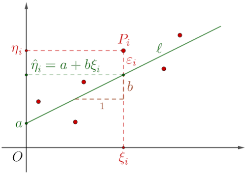
Answer: In the image on the right, the red points P1(ξ1, η1), P2(ξ2, η2), ..., Pn(ηn, ηn) are representations of random sequences:
x = (ξ1, ξ2, ..., ξn), y = (η1, η2, ..., ηn),
and Pi = (ξi, ηi) is one among them. Here, the green ℓ: $\hat{\eta} = a + b\xi$ is the regression line. It is defined so that the errors $\varepsilon_i = \eta_i - \hat{\eta}_i$ squared and summed (RSS — residual sum of squares) form the smallest value. The numb-er a is the point where the regression line intersects the ordinate, and b is the slope of the line, the tangent of its angle to the abscissa. Let the errors be nor-mally distributed 𝒩(0, σ²), expectations μ = 0 and variances σ².
1. Theorem. Given a simple linear regression model with independent readings:
$$ y = a + bx + \varepsilon, \quad \varepsilon_i \sim \mathcal{N}(0,\sigma^2), \quad i = 1, 2, ..., n. $$The parameters that minimize the residual sum of squares are given by:
$$ a = \bar{y} - b\bar{x}, \quad b = \sigma_{xy}/\sigma^2_x, $$where $\bar{x}$ and $\bar{y}$ are the sample means, and $\sigma^2_x$ is the sample variance of the data x, while σxy is the sample covariance between x and y.
Proof: The residual sum of squares is defined by:
$$ RSS(a, b) = \sum_{i=1}^n \varepsilon^2_i = \sum_{i=1}^n (\eta_i - a - b\xi_i)^2. $$The derivatives with respect to a and b of this sum are:
$$ \frac{d}{da}RSS(a,b) = -2\sum_{i=1}^n (\eta_i-a-b\xi_i) = 0, $$ $$ \frac{d}{db}RSS(a,b) = -2\sum_{i=1}^n (\xi_i\eta_i-a\xi_i-b\xi^2_i) = 0. $$We set them equal to zero because we are looking for extrema. Hence:
$$ b\sum_{i=1}^n \xi_i + an = \sum_{i=1}^n\eta_i, $$ $$ b\sum_{i=1}^n \xi^2_i + a\sum_{i=1}^n \xi_i = \sum_{i=1}^n \xi_i\eta_i. $$The first equation gives us the intersection point:
$$ a = \frac{1}{n}\sum_{i=1}^n \eta_i - \frac{b}{n}\sum_{i=1}^n \xi_i = \bar{y} - b\bar{x}. $$From the second equation we find the slope:
$$ b\sum_{i=1}^n \xi^2_i + a\sum_{i=1}^n \xi_i = \sum_{i=1}^n \xi_i\eta_i $$ $$ b\sum_{i=1}^n \xi^2_i + (\bar{y} - b\bar{x})\sum_{i=1}^n\xi_i = \sum_{i=1}^n\xi_i\eta_i $$ $$ b\left(\sum_{i=1}\xi^2_i - \bar{x}\sum_{i=1}^n \xi_i\right) = \sum_{i=1}^n \xi_i\eta_i - \bar{y}\sum_{i=1}^n \xi_i $$ $$ b = \frac{\sum_{i=1}^n \xi_i\eta_i - \bar{y}\sum_{i=1}^n \xi_i}{\sum_{i=1}^n \xi^2_i - \bar{x}\sum_{i=1}^n \xi_i}. $$Let's rewrite the numerator in the form:
$$ \sum_{i=1}^n \xi_i\eta_i - \bar{y}\sum_{i=1}^n \xi_i = \sum_{i=1}^n \xi_i\eta_i - n\bar{x}\bar{y} = $$ $$ = \sum_{i=1}^n \xi_i\eta_i - n\bar{x}\bar{y} -n\bar{x}\bar{y} + n\bar{x}\bar{y} $$ $$ = \sum_{i=1}^n \xi_i\eta_i - \bar{y}\sum_{i=1}^n \xi_i - \bar{x}\sum_{i=1}^n \eta_i + \sum_{i=1}^n \bar{x}\bar{y} $$ $$ = \sum_{i=1}^n (\xi_i\eta_i - \xi_i\bar{y} - \bar{x}\eta_i + \bar{x}\bar{y}) $$ $$ = \sum_{i=1}^n (\xi_i - \bar{x})(\eta_i - \bar{y}). $$The denominator can be rewritten in the form:
$$ \sum_{i=1}^n \xi^2_i - \bar{x}\sum_{i=1}^n \xi_i = \sum_{i=1}^n \xi^2_i - n\bar{x}^2 = $$ $$ = \sum_{i=1}^n \xi^2_i - 2n\bar{x}\bar{x} + n\bar{x}^2 $$ $$ = \sum_{i=1}^n \xi^2_i - 2\bar{x}\sum_{i=1}^n \xi_i + \sum_{i=1}^n \bar{x}^2 $$ $$ = \sum_{i=1}^n (\xi^2_i - 2\bar{x}\xi_i + \bar{x}^2) $$ $$ = \sum_{i=1}^n (\xi_i - \bar{x})^2. $$Returning these rewritten forms to the above fraction, we get:
$$ b = \frac{\sum_{i=1}^n (\xi_i - \bar{x})(\eta_i - \bar{y})}{\sum_{i=1}^n (\xi_i - \bar{x})^2} $$and when we divide the numerator and denominator by n we get:
$$ b = \frac{\sigma_{xy}}{\sigma^2_x}. $$With $a = \bar{y} - b\bar{x}$ already found, this b proves the theorem. ∎
2. The result of this theorem can be written in the form:
$$ y = a + bx, \quad a = \mu_y - b\mu_x, \quad b = r\frac{\sigma_y}{\sigma_x}, $$where μx and μy are the mathematical expectations of the sequences x and y, while σx and σy are the roots of the variances. The number r = r(x, y) is the Pearson correlation coefficient which I denoted in the "February" (previously written) blogs with κ(x, y) especially because of the interpretation of quantum entanglement (Singlet) and Bell's theorem. The following example is a conti-nuation of the example from that blog.
3. Example. Let's find a simple regression line for a series of variables:
x = (22, 35, 29, 34, 39, 42, 45), y = (12, 24, 17, 23, 29, 33, 36).
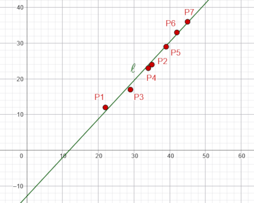
Solution: Given the arrays of points Pi(xi, yi), where i = 1, 2, ..., 7:
P1(22, 12), P2(35, 24), P3(29, 17), P4(34, 23), P5(39, 29), P6(42, 33), P7(45, 36).
In the previous blog (Boiled frog) it was already calculated:
μx = 35, μy = 25, σx = 7.28, σy = 7.92, r = 0.994.
Hence we find:
a = μy - bμx, b = rσy/σx, a = -12.85, b = 1.08.
The regression line, y = a + bx, is shown in the upper left image. ∎
4. Translating a random variable, X' = X + c, when c = const, does not change the variance, σ²[X'] = σ²[X], which measures the range around the mean, be-cause it does not change their distribution. However, the expectation changes E[X'] = E[X] + c. This further means that translating the random variables X or Y by a constant c in ordinary least squares (OLS) regression translates the regression line and changes the intercept, but its slope remains unchanged. In other words, adding a constant \(c\) to the independent variable X and/or the de-pendent variable Y shifts the regression line vertically or horizontally without affecting its slope. This will be a useful observation latter.
Globalism II » srb
Question: You say that both local divergence and global convergence are inevi-table, yet their accurate prediction is not possible?

Answer: Yes, mostly. However, alt-hough it seems absurd, as if one co-ntradicts the other, appearances are deceiving. Their agreement ca-nnot be disputed, the first implies the second and, especially impor-tant, note that such localism and globalism are two consequences of the objective uncertainty principle of my current theory of information. The question is long overdue (Globali-sm), but it will still fit well into the current topic of statistical regression and not as an appendix to the picture (I will be abstract, without specific politics).
1. We can also study random n-tuples of numbers x = (ξi) and y = (ηi) using a process that maps one to the other, B: x → y. For example, if all ξi ≠ 0 for i = 1, 2, ..., n:
$$ \begin{pmatrix} \eta_1 \\ \eta_2 \\ ... \\ \eta_n \end{pmatrix} = \begin{pmatrix} \eta_1/\xi_1 & 0 & ... & 0 \\ 0 & \eta_2/\xi_2 & ... & 0 \\ ... & ... & ... & ... \\ 0 & 0 & ... & \eta_n/\xi_n \end{pmatrix} \begin{pmatrix} \xi_1 \\ \xi_2 \\ ... \\ \xi_n \end{pmatrix} $$This matrix equation, Bx = y, with a diagonal matrix B of type n×n has the determinant:
$$ \det B = \frac{\eta_1}{\xi_1}\cdot\frac{\eta_2}{\xi_2}\cdots\frac{\eta_n}{\xi_n} $$which is the product of the eigenvalues λ1 = η1/ξ1, λ2 = η2/ξ2, ..., λn = ηn/ξn. We know that the eigenvalues do not change in the "similar" matrix C = P-1BP, where P and P-1 are inverse matrices, but in similar matrices the correspondi-ng eigenvectors don't have to be the same. The random sequences x and y fr-om the previous example (Least squares, 3) would have this determinant of approximately 0.069.
Through two given points, the vertices of the vectors x and y, it is possible to draw one and only one line, z = (y - x)t, of parameter t ∈ ℝ, but there are co-untless linear operators, such as C, that map x to y. Moreover, when we use only similar operators, equal sets of eigenvalues, there are still infinitely many of them with different associated eigenvectors. This is a contribution to the diversity of the paths of global convergence (Approaching).
2. When we shift the linear regression graph from the previous example by |a|, rounded to 13, so that y' = y + 13, the new line passes through the origin. We increase each ordinate by 13, so we have:
x = (22, 35, 29, 34, 39, 42, 45), y = (12, 24, 17, 23, 29, 33, 36), y' = (25, 37, 30, 36, 42, 45, 49).
The diagonal elements of the above matrix, y = B'x, and the eigenvalues λi are changed. Their new product is then det B' ≈ 1.69. The seventh root of those seven factors will be about 1.08, the slope of the regression line (b = 1.08).
In general, ξi do not change, but each η'i = ηi - a. We subtracted the intersect-ion point a = -12.85, which is negative. Therefore, the new mean value is:
$$ \bar{y}' = \frac{\eta'_1 + \eta'_2 + ... + \eta'_n}{n} = $$ $$ = \frac{(\eta_1 - a) + (\eta_2 - a) + ... + (\eta_n - a)}{n}, $$ $$ \bar{y}' = \bar{y} - a. $$We write that as μy' = μy - a. As it is (we read from the example):
$$ a = \mu_y - bμ_x = (\mu_{y'} + a) - b\mu_x, $$ $$ \mu_{y'} = b\mu_x, $$so b = μy'/μx. When the correlation of these random sequences is large, such as this r = 0.994, the quotient μy'/μx becomes approximately the nth root of the aforementioned determinant. Hence the large coincidence of the results (det B' ≈ bn).
3. Points (ξi, ηi) with infinitely increasing i = 1, 2, 3, ..., which we previously separated into partial sequences x = (ξ1, ξ2, ξ3, ...) and y = (η1, η2, η3, ...) app-ear randomly, taking only n of their members. We have no way of predicting around which point (ξ0, η0) they will cluster, and that is the principle of this theory. Those random events that are objectively uncertain cannot be predic-ted by any guesswork, forecast, calculations or measurements, nor will it ever be possible until their realization.
This is local divergence. It then implies that even the linear regression of the aforementioned infinite sequences cannot be known on the basis of their par-tial subsequences. Especially because of adaptations in real situations, which say that each new occurrence affects at least some small part of the continua-tions of the previous ones. The force of uncertainty transmitted through the appearance of a new coincidence (a point, therefore a vector, or a state) cons-tantly changes the previous regression line and the direction of globalization, unknowably. This is the way in which local divergence makes global conver-gence unpredictable. It is encouraged by the law of large numbers of proba-bility theory, but in another way by linear algebra.
Python program » srb
Question: Send me the Python code for linear regression?
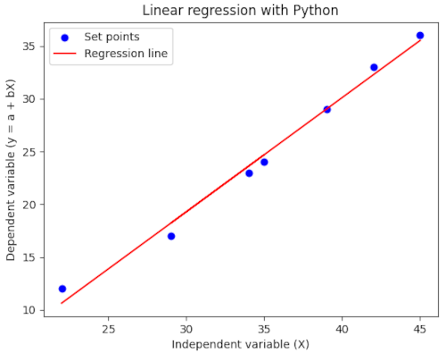
Answer: In the image on the left you see the result of the program from the following. The data is the previous one:
x = (22, 35, 29, 34, 39, 42, 45) y = (12, 24, 17, 23, 29, 33, 36)
The coefficient of determination (r²) is just the square of the Pears-on r(x, y) correlation coefficient; it means the proportion of the varia-tion in the dependent variable y that is predicted based on the in-dependent variable. The equation y = a + bx is the line that intercepts the ordinate at elevation a and has slope b, otherwise the tangent of the angle to the abscissa. Additionally, based on the new abscissas X = (10, 20, 30) the predicted ordinates are y = (-2.33898305, 8.47765794, 19.29429892) as a bonus. Python (3.11.0):
# pip install numpy pandas matplotlib scikit-learn
from sklearn.linear_model import LinearRegression
import matplotlib.pyplot as plt
import numpy as np
# Sample data, reshape to a 2D array
X = np.array([22, 35, 29, 34, 39, 42, 45]).reshape((-1, 1))
y = np.array([12, 24, 17, 23, 29, 33, 36])
model = LinearRegression()
model.fit(X, y)
r_sq = model.score(X, y)
print(f"Coefficient of determination (r^2): {r_sq}")
print(f"Intercept (a): {model.intercept_}")
print(f"Slope (b): {model.coef_}")
# Prediction based on existing data
y_pred = model.predict(X)
# Forecasting on the basis of new data
x_new = np.array([10, 20, 30]).reshape((-1, 1))
y_new_pred = model.predict(x_new)
print("Forecasting new ones, for X = (10, 20, 30):")
print("y =", y_new_pred)
# drawing
plt.scatter(X, y, color='blue', label='Set points')
plt.plot(X, y_pred, color='red', label='Regression line')
plt.xlabel('Independent variable (X)')
plt.ylabel('Dependent variable (y = a + bX)')
plt.title('Linear regression with Python')
plt.legend()
plt.show()
At the beginning it is stated (pip install ...) how to install the Python module from the computer's command mode, if you don't have it. I further modestly stated the comments (they start with #) to make it easier to understand what the program does, without overloading it too much. In addition to the draw-ing, at the top left, the program also gives the following text on the screen:
Coefficient of determination (r^2): 0.9887085901386748
Intercept (a): -13.155624036979983
Slope (b): [1.0816641]
Forecasting new ones, for X = (10, 20, 30):
y = [-2.33898305  8.47765794 19.29429892]
Modify the program to suit your needs. The same version as the module is here.
Spline » srb
Question: Can you explain to me in a little more detail how you build linear operators using the “joins”?
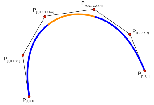
Answer: This is part of a discussion about the stereometry of statistics (Restriction) called there joints, or "splines" (novelty and I don't have a better name), which somewhat resemble these images on the right, hence the confusion.
1. I will explain step by step, so that we do not confuse this new conce-pt, here "joints" $\vec{s}_x$, with something already known and do not get lost. First of all, we have a n-tuple of numbers x = (ξ1, ..., ξn), whose elements ξi are random (or some other) numbers with mean value μx = (ξ1 + ... + ξn)/n. With such we form the joins Sx = (ξ1-μx, ..., ξn-μx), sequences which are also vectors. In the figures in the quotation we see them as "rejections" of the projections of the vector $\vec{x}$ onto the quadrant bisector to the given vector. They are perpendi-cular to these bisectors, and the cosines of the angles between the joins are eq-ual to the (Pearson) correlation coefficients.
2. The scalar product of two joins:
$$ \vec{S}_x\cdot\vec{S}_y = (\xi_1 - \mu_x)(\eta_1 - \mu_y) + ... + (\xi_n - \mu_x)(\eta_n - \mu_y) = n\,\text{cov}(x,y) $$is the n times increased covariance of the corresponding sequences x and this y = (η1, ..., ηn), the other with mean μy = (η1 + ... + ηn)/n. Again, the covarian-ce is the mean of that scalar product. Next, we have the variances:
$$ \sigma^2_x = \frac{1}{n} \sum_{i=1}^n (\xi_i - \mu_x)^2, \quad \sigma^2_y = \frac{1}{n} \sum_{i=1}^n (\eta_i - \mu_y)^2 $$from which the intensities of the joins vectors, dispersions:
$$ \sigma_x = \frac{1}{\sqrt{n}}\|\vec{S}_x\|, \quad \sigma_y = \frac{1}{\sqrt{n}}\|\vec{S}_y\|. $$The scalar product of the coefficients divided by these variances is the Pearson correlation coefficient of the x and y series:
$$ \frac{\vec{S}_x}{\sigma_x}\cdot \frac{\vec{S}_y}{\sigma_y} = r(x,y), $$in the aforementioned article marked with κ(x, y). The continuation of this story is even more disturbing, so I just need to slow down that part of the presentation.
3. Joins, or “splines”, are sequences with a zero mean:
$$ \mu_s = \frac{1}{n}[(\xi_1 - \mu) + ... + (\xi_n - \mu)] = $$ $$ = \frac{1}{n}[(\xi_1 + ... + \xi_n) - (\mu + .. + \mu)] $$ $$ = \frac{1}{n}(\xi_1 + ... + \xi_n) - \frac{1}{n}(n\mu) $$ $$ = \mu - \mu = 0. $$Therefore, joins, like "ordinary" sequences, can be considered states, and so-metimes interpretations of similar vectors. Their inner (scalar) products can represent information of perception, and we can also talk about their linear regressions.
4. The translation (Least squares, 4) of the linear regression, y = a + bx, does not change its slope b, so by parallel shearing it vertically we can reduce it to the form (y - a = bx) when it passes through the origin. On the other hand, it is known that b = rσy/σx, so applied to linear regressions of joints we have:
$$ \vec{S}_y = \frac{1}{n}\frac{\vec{S}_x\cdot\vec{S}_y}{\sigma_x\sigma_y}\frac{\sigma_y}{\sigma_x}\vec{S}_x, $$because the joins have zero mean (3). We can write this:
$$ \vec{S}_y = \frac{\vec{S}_x\cdot\vec{S}_y}{\|\vec{S}_x\|\|\vec{S}_y\|}\frac{\|\vec{S}_y\|}{\|\vec{S}_x\|}\vec{S}_x, $$ $$ \frac{\vec{S}_y}{\|\vec{S}_y\|} = \frac{\vec{S}_x\cdot\vec{S}_y}{\|\vec{S}_x\|\|\vec{S}_y\|}\frac{\vec{S}_x}{\|\vec{S}_x\|}, $$ $$ \vec{s}_y = (\vec{s}_x\cdot\vec{s}_y)\, \vec{s}_x, $$where $\vec{s}_x$ and $\vec{s}_y$ are the unit vectors of the joins $\vec{S}_x$ and $\vec{S}_y$.
5. The next step is to apply this to linear operators, because they also have the properties of vectors. Thus we arrive at the aforementioned "construction" of operators by joins, from the discussion and the question posed, but which is a separate topic of linear algebra. States are representations of vectors made up of sequences of independent properties of different strengths of manifestation. If we understand interactions as communications, then scalar products appear as information of perception. Thus these vectors become topics of physics and information theory.
Furthermore, the point is that processes are interpretations of operators, and “process states” are a special form of them that can also be understood as an ordinary vector, say a series or a directed length like speed or force. Moreover, the process of time, due to the “force of probability”, will behave as a “pushi-ng” of physical (static) states into the future and will correspond to the prop-erties of a vector. Its form is vector and what we can extract from the vector calculus we transfer to the interpretation.
Magnitude » srb
Question: What could be said about such an interpretation of linear regression (Spline, 4), with a slope b that is not a number?
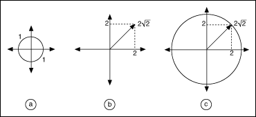
Answer: We're going beyond the framework of classical statistics and we don't look at those formulas in those ways. That's the first. To continue, I'm working on linear algebra, then on the related area of functional analysis. I can briefly outline some of that.
1. In that image, on the top left, is a link with an explanation of the transfer of the norm of vectors to the norm of the matrix that maps them. In the 2-norm of vectors (Euclidean), the root of the sum of the squares of the elements of the vector x = (ξ1, ..., ξn) is its intensity, so that norm is simply the factor by which we must multiply the unit ball so that the vector x remains in it:
$$ \|x\|_2 = \sqrt{|\xi_1|^2 + ... + |\xi_n|^2}, \quad \xi_1, ..., \xi_n \in \mathbb{C}. $$The corresponding norm of an operator measures the maximum "stretch" that it applies to any vector space on which it acts. The same is true for matrices that are interpretations of the operator in various bases of that space. Precise-ly, we say that a (linear) operator A in a vector space X is bounded if there exists a non-negative number M such that:
$$ \|Ax\| \le M\|x\|, \quad \forall x \in X. $$The infimum of the numbers M (the smallest of them, or limit) is the norm of the operator A. An operator is therefore bounded if it has a finite norm, and then:
$$ \|Ax\| \le \|A\|\|x\|, \quad \forall x \in X. $$When unlabeled, we assume Euclidean norms.
2. When we use only unit vectors of the same space, the norm of the operator is:
$$ \|A\| = \sup_{x\in X\setminus\{0\}} = \frac{\|Ax\|}{\|x\|} = \sup_{\|x\|=1}\|Ax\|, $$so the norm of the operator is bounded by the norm of the mapped unit vect-ors. Since the connectors in the above equation are unit vectors, we write this (Spline, 4) as $\vec{s}_y = A\vec{s}_x$ and note that the norms of this regression are unit, $\|A\| = 1$. Since $\vec{s} = \vec{S}/\|\vec{S}\|$, and the denominator is proportional to the dispe-rsion σ (and the root of the constant number of components), the connectors Sx are mapped to larger Sy such that their dispersions σy grow proportionally. The reverse is also true, shorter connectors will have smaller dispersions.
3. If we take the raw (unnormalized) joins and the corresponding mappings of the slope coefficients of the regression line into the operator, b = rσy/σx → B, and because |r| ≤ 1 and the previous ∥A∥ = 1, it follows σy ≥ σx. This growth speaks of the tendency of dilution of random events in my interpretation of supposedly linear regression. This is a bit of a long story (for this occasion) and I will only state that it goes with the noise of the Markov chain, the info-rmation carrier channel, which is created by excess information, therefore, with an increase in uncertainty and dispersion of messages.
4. Treating this problem with a determinant is a completely different story, al-so interesting but separate. Namely, look at these two simple matrices whose determinants are one (det C1 = det C2 = 1):
$$ C_1 = \begin{pmatrix} 1 & c \\ 0 & 1 \end{pmatrix}, \quad C_2 = \begin{pmatrix} \sqrt{1 + c^2} & c \\ c & \sqrt{1 + c^2} \end{pmatrix} $$but when c → ∞, then ∥Cx∥ → ∞ for many vectors x. Otherwise, the determina-nt is a scalar (real or complex number) for square matrices, that will tell whe-ther the matrix can be inverted (the determinant is then nonzero) and how much it scales the volume/area, but there is no rule that the norm must be gr-eater than the determinant (or vice versa).
Entropy III » srb
Question: I just noticed a novelty, how does linear regression itself reveal spo-ntaneous growth of entropy?
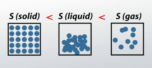
Answer: Yes, you saw that clearly from the previous answer. The re-gression line, y = a + bx, shifted parallel changes the point of inte-rsection with the ordinate a, but does not change the slope which is b = rσy/σx. Shifted so that a = 0, it will be y = bx and then the effect of the coefficient b, from the independent random variable x to the dependent y, can be seen better. The coefficient r ∈ [-1, 1] shows the correlation of the vari-ables x with y, and σx and σy are their dispersions, the roots of the variances.
You have noticed (Magnitude, 3) that by applying the above to the joins Sx and Sy, and this is especially visible after their normalization, we have σx ≤ σy, be-cause |r| ≤ 1. This means that the dispersion of the dependent variable tends to increase. Like entropy, about whose official version I have a separate opini-on and which I have mentioned several times, in these blogs (Entropy II), in a little more detail (Entropy), or earlier (Information of Perception, p. 79).
1. When we don't have enough data, we are uninformed, but if we are too info-rmed, we are misinformed. Unlike dead physical nature, vitality is an addition that gives us greater choices, that we don't have to follow the principle of least action, but also that we can lie. That's the difference between physics and info-rmation theory. The former doesn't deal with lies and can only partially under-stand entropy.
The needle is well hidden in a haystack (Unaffected, 2). Similarly, interference in data transmission, which can also be traced to Markov chains (Black Box II), starts by suffocating the "right" information with the "wrong", that is, by saturating the sent message. The sent message does not actually disappear, it is buried and ignored, unrecognizable. We can also observe this "unusual" ph-enomenon within classical physics in the pursuit of the status quo. The least action is not something that goes to zero and below, but encounters equilibri-um positions, optima, on its way. Too much decrease in physical action and too little are equally repulsive to bodies in motion.
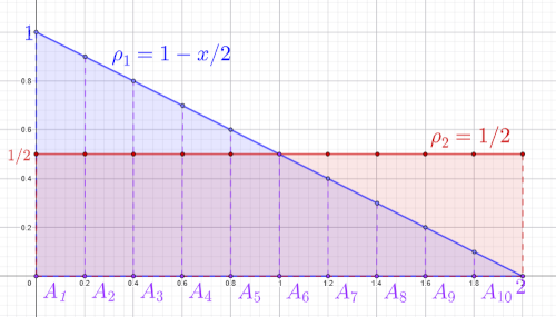
2. The figure on the left shows two probability density graphs, for x ∈ [0, 2]:
$$ \rho_1(x) = 1 - \frac12x, \quad \rho_2(x) = \frac12, $$and ρ1(x) = ρ2(x) = 0 for x ∉ [0, 2]. And the area of a right triangle with sides 1 and 2 below the hypotenuse (blue) to the abscissa is 1⋅2/2 = 1. Also, the area of a (red) rectangle with sides 1/2 and 2 is 1. Therefore, they describe probability distributions in this way.
3. The Shannon information of the first density is significantly smaller than the second:
$$ S_1 = -\int_0^2 (1 - \frac12x)\ln(1 - \frac12x)\,dx = \int_1^0 2y\ln y\,dy = $$ $$ = \int_1^0 \ln y\,dy^2 = y^2\ln y\Bigg|_1^0 - \int_1^0y^2\,d\ln y $$ $$ = -\int_1 ^0y^2\cdot \frac{1}{y}\,dy = -\int_1^0 y\,dy $$ $$ = -\frac{y^2}{2}\Bigg|_1^0 = \frac12 = 0.5. $$Here the substitution used is y = 1 - x/2, so x = 2 - 2y. However, the Shannon information of the second density is:
$$ S_2 = -\int_0^2 \frac12 \ln\frac12\, dx = (\frac12 \ln 2) \, x\Bigg|_0^2 = \ln 2 \approx 0.69. $$4. Ten events A1, ..., A10 arranged along the abscissa, according to the first density have decreasing probabilities in that order. The first A1 is the most probable and occurs most often (repeatedly), but if it does happen, it is not news. The second density ρ2 has a uniform distribution and each of the ten given events is equally (un)expected, each is equally masked by the remaining nine and therefore its information is greater, but it is impersonal, disordered. It is one of the examples of how entropy with its disorder reduces (useful) in-formation, which I sometimes use to see that as entropy increases we lose information about specific data.
Karma II » srb
Question: Does entropy thus defy principled minimalism?

Answer: This linear regression indicates a possible spontaneous increase in dispersion, and with it "disorder", or entropy in the class-ical sense, but there is a noticeable (Entropy III, 2) drop in the expo-sure of each individual message, including significant ones. In other words, noise drowns out informati-on, so if we view disorder as a spo-ntaneous increase in information, we should also see its spontaneous decrease in it.
1. Efficiency is the release of excess choices (Unaffected, 2), because in real ti-me it is not productive to check too much for the reliability, accuracy of items or the reality of phenomena, so at best this oversaturation leads us to rough estimates and inevitable errors. The ultimate reaches of intelligence are then limited by deception (Mastery). However, the paths of deception quickly be-come a fall from the train of reality that does not care about lies and leaves them behind in a ditch by the wayside, and in the end reality and truth are the only indestructible ones. They survive and that is how we distinguish them from fictions. In this way, too, increasing dispersion does not mean greater information. As if by some kind of karma, bad decisions can punished us and excess freedom can be turned into a deficit in a bad way.
2. We distinguish between internal and external information (In and Out), with the former becoming attenuated when magnified, and what we see at longer wavelengths (position uncertainties) in their poorer interaction with the environment, we call it greater penetration. Also, a body of faster relative motion interacts more frequently with our same environment, is oversaturat-ed with information, and part of such a system is in a parallel reality, in addi-tional dimensions of time. It is similar to gravity, where we also observe a slo-wdown in the flow of time, here understood by the way of finding it observed both in our and in pseudo-reality. What we see in these situations are losses of information due to the increase in entropy.
3. In the short term, the increase in entropy, in the form of disorder, may resemble an increase in the amount of possibilities (information), but in the long term, entropy is dissipation and cooling, a loss of content and dynamics. In the end, it also becomes a loss of interactions, or communication. In this sense, the pieces of glass, a beaker that fell from the table and broke, are made impersonal and like a parade of soldiers who still contain their individual cha-racteristics and differences on the inside, but do not show them on the outsi-de. Entropy, during its spontaneous increase, loses active information and in its own way testifies to the principle of minimalism.
Dual » srb
Question: The subject and the object do not see the common space equally?
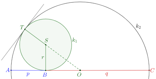
Answer: Yes, their perceptions are different in various ways. This inc-ludes differences in dual percepti-ons of the same space. Then they have different metrics:
$$ d(x,y) = [\sum_{i=1}^n (\xi_i - \eta_i)^a]^{1/a} $$when the points of the n-tuple are x = (ξ1, ..., ξn) and y = (η1, ..., ηn). But, if in one space a = p > 1, then in the dual a = q, where:
$$ \frac{1}{p} + \frac{1}{q} = 1. $$These two metrics are equal only if p = q = 1/2, and this is only the case in the Euclidean 2-norm metric.
1. We see such numbers (r = 1) in the previous image, top left:
$$ \frac{1}{p} + \frac{1}{q} = \frac{1}{r}. $$A smaller circle k1 with center S and radius r is inscribed in a semicircle k2 with center O and radius p + q with points of contact T and B. Point B divides the diameter into two parts AB = p and BC = q, and the tangent at point T is perpendicular to the diameters of both circles, so T-S-O, these are three coll-inear points with the center of the smaller circle between them. To prove the above equality, we have the right triangle SBO:
$$ SB^2 + BO^2 = OS^2, $$ $$ r^2 + \left(\frac{b-a}{2}\right)^2 = \left(\frac{a+b}{2}-r\right)^2, $$and after squaring and arranging we find the required equality.
2. The figure shows that when the smaller circle (k1) with center (S) approach-es the edge of the diameter (A), it decreases. Since its radius is always the sa-me (r = 1), this means that the diameter (p + q) of the larger semicircle (k2) increases. In this case, p → r = 1, which means that q → ∞. One of the (less-known) examples of such dual metrics is the space of probability and inform-ation (Dual Likely):
$$ d_1(x,y) = |\xi_1 - \eta_1| + ... |\xi_n - \eta_n|, $$ $$ d_\infty(x,y) = \max\{|\xi_1 - \eta_1|, ..., |\xi_n - \eta_n|\}. $$This is the case in classical theory when we add probabilities directly, as non-negative real numbers from the interval from 0 to 1. Then news of rare events dominate (it is not as much news when a dog bites a man as when a man bites a dog), so the leading ones are the largest, maximal ones. Namely:
$$ \|x\|_\infty = \lim_{a \to \infty}\left(|\xi_1|^a + ... + |\xi_m|^a + ... + |\xi_n|^a\right)^{1/a} = $$ $$ \lim_{a \to \infty}|\xi_m|\left(|\frac{\xi_1}{\xi_m}|^a + ... + |\frac{\xi_m}{\xi_m}|^a + ... + |\frac{\xi_m}{\xi_n}|^a\right)^{1/a} = |\xi_m|, $$where ξm is the absolute largest coordinate of the sequence x, so the expressi-on in parentheses is 1, i.e.
$$ \|x\|_\infty = \max_{1\le i\le n} \{|\xi_i|\}. $$However, in quantum physics probabilities are 2-norms (Born's rule), and so is information. Dualism is also evidenced by the interesting dispute between Protagoras and Euathlus (Dual Power).
3. The scalar (or inner) product induces a norm (\(||x||=\sqrt{\langle x,x\rangle }\)) if and only if the norm satisfies the parallelogram law:
$$ ||x+y||^{2}+||x-y||^{2}=2||x||^{2}+2||y||^{2}. $$For p-norms $|x||_{p}=(\sum_i |x_{i}|^{p})^{1/p}$, the norm induces a scalar product if and only if p = 2 (the Euclidean norm). This is because the scalar product is an equal mixture of the factors of both mutually dual spaces (Restriction):
$$ \langle s_x | s_y\rangle = (\xi_1 - \mu_x)(\eta_1 - \mu_y) + ... + (\xi_n - \mu_x)(\eta_n - \mu_y). $$We know that for such splines that μx and μy are the mean values of the sequ-ence x = (ξi) and y = (ηi), so the covariance is:
$$ \text{cov}(x,y) = \frac{1}{n}\langle s_x|s_y\rangle, $$regardless of the type of dualism. This is an arbitrary (my) declaration and is not worth looking for in textbooks, but it works and does not contradict the known!
4. However, the standard deviations are isolated, so we use duals:
$$ \sigma_x = \left[\frac{1}{n}\sum_{i=1}^n(\xi_i - \mu_x)^p\right]^{1/p}, \quad \sigma_y = \left[\frac{1}{n}\sum_{i=1}^n(\eta - \mu_x)^q\right]^{1/q}, $$where p-1 + q-1 = 1. Next, we define Pearson's correlation:
$$ \kappa(x,y) = \frac{\text{cov}(x,y)}{\sigma_x\sigma_y} = \frac{\sum_{i=1}^n (\xi_i - \mu_x)(\eta_i - \mu_y)}{\left[\sum_{i=1}^n (\xi_i - \mu_x)^p\right]^{1/p} \left[\sum_{i=1}^n (\eta_i - \mu_x)^q\right]^{1/q}}, $$ $$ \kappa(x,y) = \frac{\langle s_x | s_y\rangle}{\|s_x\|_p\, \|s_y\|_q}, $$because n in the numerator is reduced to n1/pn1/q = n in the denominator. This is the correlation coefficient of the now dual spaces. If we put p = q = 2, we get its previously known form, here as a special case.
5. With a larger number p > 1, the p-norm is smaller. This is obvious for ∥x∥∞ ≤ ∥x∥p, because on the left is the largest absolute, say |ξm|, of the series terms x = (ξ1, ..., ξn), and on the right there are more of them in the sum, so it is certain:
$$ |\xi_m| \le \left(|\xi_1|^p + ... + |\xi_m|^m + ... + |\xi_n|^p\right)^{1/p}. $$In general:
$$ \|x\|_q = \left(\sum_{i=1}^n |\xi_i|^q\right)^{1/q} = \left(\sum_{i=1}^n |\xi_i|^{q-p}\,|\xi_i|^p\right)^{1/q} \le $$ $$ \le \left(\sum_{i=1}^n |\xi_m|^{q-p}\,|\xi_i|^p\right)^{1/q} = |\xi_m|^{(q-p)/q} \left(\sum_{i=1}^n |\xi_i|^p\right)^{1/q} $$ $$ = |\xi_m|^{(q-p)/q} (\|x\|_p)^{p/q}, $$ $$ \|x\|_q \le \|x\|_p, \quad p \le q. $$Smaller values of p (e.g. ∥x∥1) give more weight to small errors, while larger values of p (e.g. ∥x∥∞) dominate by their largest components, making them smaller overall compared to the sum of all elements. In short, it is a descrip-tion of what these norms do to random sequences.
Hölder » srb
Question: What about the denominator of the correlation, what is the magnit-ude of the product of the dual norms?
Answer: This follows directly from Helder's inequality Quantum Mec-hanics (Theorem 1.3.3, p. 192). For any two sequences x = (ξi) and y = (ηi) and p-1 + q-1 = 1, the following holds:
$$ |\langle x | y\rangle| \le \|x\|_p\|y\|_q. $$In the case of correlation, hence:
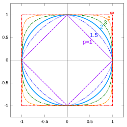
$$ \kappa(x,y) = \frac{\langle s_x|s_y\rangle}{\|s_x\|_p\, \|s_y\|_q} \le 1, $$when 1/p + 1/q = 1, because the above also applies to the case of joins, and therefore also to Pearson's correlation. The picture shows examples of such p-norms for p ∈ {1, 1.5, 2, 3, 6, ∞} where we can more easily see how these norms deform the unit circle ∥x∥p = 1. There are much more interesting explanations of dual spaces, possibly suitable for some occasions, and here let's just look at how a straight line changes using another the p-norm.
1. The correlation is still equal to the cosine of the angle between the splines of two random sequences, $\kappa(x,y) = \cos\angle(\vec{s}_x,\vec{s}_y)$, and the linear regression line y = a + bx. When converted to polar coordinates, it becomes x = r⋅cos(φ) and y = r⋅sin(φ), so we have:
$$ r\sin\varphi = a + br\cos\varphi, $$ $$ r(\sin\varphi - b\cos\varphi) = a, $$ $$ r(\sin\varphi\cos\beta - \cos\varphi\sin\beta) = a\cos\beta, \quad b = \tan\beta, $$ $$ r = \frac{a\cos\beta}{\sin(\varphi-\beta)}. $$This is the equation of a line in 2-norm (Euclidean), as we usually know it. The angle β is between the line and the abscissa.
2. In an arbitrary p-norm (p ≥ 1), we further have:
$$ (x^p + y^p)^{1/p} = \frac{a\cos\beta}{\sin(\varphi-\beta)}, $$ $$ r(\cos^p\varphi + \sin^p\varphi)^{1/p} = \frac{a\cos\beta}{\sin(\varphi-\beta)}, $$ $$ r = \frac{a\cos\beta}{\sin(\varphi-\beta)}\frac{1}{(\cos^p\varphi + \sin^p\varphi)^{1/p}}. $$This equation reduces to the Euclidean equation for p = 2, because the sum of the squares of the cosine and sine is one. However, the p-norm is smaller wh-en p is a larger, so this r is larger. The upper line then moves away from the origin.
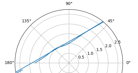
3. In the image on the left, the stra-ight line y = 1 + tan(π/6)x in 3-no-rm is plotted in Python. We can see that it passes slightly above the 1 of ordinate and that it slightly undula-tes around the straight line. In the norm p = 2, it is a straight line that intersects the ordinate at the height a = 1 and has a slope b = tan(30°), which means that it makes an angle of 30 degrees with the abscissa (the horizontal, usually x axis).
4. These are not problems from spatial distribution, nor from the calculation of Christoffel symbols, but from a completely different milieu, say, the follow-ing (Real Life). Let's compare the amount of time spent studying with the test results: number of study hours 2, 4, 6; test result 50, 70, 90. We will get the equation y = 30 + 10x which would be what we are looking for if it were not too exact for statistics. Linear regression questions also require significant amounts of uncertainty in these numbers, which are not present in the motion of celestial bodies or in the theorems of Thales.
Multilinear » srb
Question: Can you also say something about multiple linear regression?
Answer: Simple regression is the relationship between one depende-nt (y) variable and one independe-nt (x) variable:
y = f(x).
Multiple regression (with many variables) is a function of one dependent variable with many independent variables:
y = f(x1, x2, ..., xn).
Multivariate regression refers to multiple dependent but also mul-tiple independent variables:
y1, y2,..., yn = f(x1, x2, ..., xn).
I assume the one you're asking about is this intermediate one, called multiple and linear, or multilinear:
Y = X1 + X2 + ... + Xn
with random variable Xi in order for all i = 1, 2, ..., n.
1. It is a regression that implies four prerequisites: (1) The relationships betw-een the dependent and independent variables are linear; (2) The variance of the errors is equal for all independent variables, this is called homoscedastic-ity; (3) The residuals follow a normal distribution; (4) The independent vari-ables should not be highly correlated, they are not close to +1 or -1.

2. It, like correlation, suffers many times more from the "diseases" of simple regressions. For example, from false correlations, coincide-nces that are clearly not causal. Those in the picture on the left are the frequency of giving babies the name Marquis in the USA with robberies in Kansas, correlation index r = 0.948.
The randomness of the variables of one n-tuple and another n-tuple will coi-ncide in the extent of the correlation of this index (r ≥ 0.94) with decreasing probabilities as n becomes a larger number, but with the growing number of all kinds of statistical measurements around the world today, it can absolutely increase. What if independent variables, such as the aforementioned Marquis babies and the Kansas robberies, show a correlation even though there is no causality? What then about the findings of multiple regression, and especially if we are not sure that something is just a correlation (mere coincidence) and not something more (causality). This possibility does not reduce, but rather increases the difficulties of multiple regression.
3. Another example, ice cream and drowning. A regression of drowning incid-ents on ice cream sales will show a strong positive correlation suggesting that ice cream causes drowning! But adding “temperature” as a control variable in a multilinear model reveals that high temperatures cause both, removing the absurd cause-and-effect relationship.
A similar instructive example occurred at UC Berkeley in 1970 during the uni-versity's admissions process. The data indicated a bias against women in adm-issions. However, a multilinear regression controlling for department did not show any bias, revealing that women applied to more competitive departmen-ts.
4. Unofficially, only in this theory of information, reality, truthfulness and su-stainability are in the same category of concepts, indestructible, that is, resist-ant to the passage of time. If we compare them with Gödel's second theorem, which states that mathematics cannot prove itself (Dogma), an unusual obse-rvation arises. When we are not able to discover a contradiction, or definitive proof of falsity, we are condemned to observe the duration of given states (st-atements, phenomena, flows) hoping that they will subside. Until such times, it is not wrong to keep them in the category of "truths", alleged like some trai-nees. Unlike lies, truth is what lasts, also what would consistently show supe-rior correlation with more and more random variables in a suitable multiline-ar regression.
Reckoning » srb
Question: Do you have any real examples of these linear regressions?

Answer: Let's take public data from the Statistical Office of the Republi-ka Srpska, now in CSV format:
Year,Population,Pupils,PPC
2014,1167082,43975,3904
2015,1162164,42089,4058
2016,1157516,41136,4263
2017,1153017,40035,4478
2018,1147902,38499,4766
2019,1142495,37206,5035
2020,1136274,36405,5009
2021,1128309,35615,5665
2022,1120236,34998,6635
2023,1114819,34825,7378
2024,1110496,35118,7922
which I saved in a teka.csv file with an Excel-like program (WPS Office) in the folder with the Python program. As you can see, they (Comma-Separated Val-ues) are, by year (Year) from 2014 to 2024, the number of inhabitants (Popu-lation), total secondary school students (Pupils) and gross product per capita in euros (PPC). Here they are in the picture, top right.
1. For simple correlations, all at once, we have a Python program:
import pandas as pd
df = pd.read_csv('stat.csv')
print(df.corr())
prints the Pearson correlation coefficients of all pairs on the screen:
                Year  Population    Pupils       PPC
Year        1.000000   -0.995927 -0.966720  0.949583
Population -0.995927    1.000000  0.949351 -0.966436
Pupils     -0.966720    0.949351  1.000000 -0.846598
 PPC        0.949583   -0.966436 -0.846598  1.000000
This means, in the first row of numbers, that year-year have a correlation coef-ficient of 1.000 but year-population -0.996. As years grow, the population de-creases, and so does the number of students (-0.967), but per capita income increases (0.950).
2. Finding a multiple regression, here two of Year, Population, Pupils and PPC, is looking for a linear structure, of the form y = β0 + β1⋅X1 + β2⋅X2. Say we are glance the fourth y = PPC for which we are looking the β0 = Intercept with coefficients β1 and β2 of which the factors are the first two independent variables mentioned. The following program finds them and a few more:
import pandas as pd
import numpy as np
from sklearn.linear_model import LinearRegression
from sklearn.model_selection import train_test_split
from sklearn.metrics import mean_squared_error, r2_score

data = {'Year': [2014, 2015, 2016, 2017, 2018, 2019, 2020,
                 2021, 2022, 2023, 2024],
        'Population': [1167082, 1162164, 1157516, 1153017,
                       1147902, 1142495, 1136274, 1128309,
                       1120236, 1114819, 1110496],
        'Pupils': [43975, 42089, 41136, 40035, 38499,
                   37206, 36405, 35615, 34998, 34825, 35118],
        'PPC': [3904, 4058, 4263, 4478, 4766, 5035, 5009,
                5665, 6635, 7378, 7922]}
df = pd.DataFrame(data)
print(df)
X = df[['Year', 'Population']]  # Multiple independent variables
y = df['PPC']                 # Dependent variable as a Series
X_train, X_test, y_train, y_test = train_test_split(X, y,
                        test_size=0.3, random_state=100)
model = LinearRegression()
model.fit(X_train, y_train) # Fits the model to the training data
print('Intercept:', model.intercept_)
print('Coefficients:', model.coef_)
y_pred = model.predict(X_test)
print(f"\nPredicted responses for test set: {y_pred}")
mse = mean_squared_error(y_test, y_pred)
r2 = r2_score(y_test, y_pred)
print(f"\nMean Squared Error (MSE): {mse}")
print(f"Coefficient of Determination (R-squared): {r2}")
By running this program, the following appears on the screen:
    Year  Population  Pupils   PPC
0   2014     1167082   43975  3904
1   2015     1162164   42089  4058
2   2016     1157516   41136  4263
3   2017     1153017   40035  4478
4   2018     1147902   38499  4766
5   2019     1142495   37206  5035
6   2020     1136274   36405  5009
7   2021     1128309   35615  5665
8   2022     1120236   34998  6635
9   2023     1114819   34825  7378
10  2024     1110496   35118  7922
Intercept: 840802.4525575939
Coefficients: [-3.43030412e+02 -1.25276613e-01]

Predicted responses for test set: [7191.18021636
	5532.46173013 4004.20229184 5096.14633552]

Mean Squared Error (MSE): 78886.72055445887
Coefficient of Determination (R-squared): 0.9473733650695393
So, the coefficients (β0, β1, β2) are:
(840802.4525575939, -343.030412, -0.125276613)
So, the formula to calculate PPC is:
ppc14 = β0 + β1⋅2014 + β2⋅1167082 ≈ 3731 [3904], ppc15 = β0 + β1⋅2015 + β2⋅1162164 ≈ 4004 [4058], ppc16 = β0 + β1⋅2016 + β2⋅1157516 ≈ 4243 [4263], ...
In square brackets on the right, the PPC (Product per Capita) data is measured.
3. Many populations in the world confirm that the growth of per capita output has an opposite trend to natural increase, the birth rate, but this is not pretty new. Having children is harmful to the modern economic prosperity of socie-ty, and nature has its own mechanisms against pests that we rarely understa-nd, and even the side that does not resist them loses (Pest). This is supported by the game theory of this information theory (Traits) with one surprising (hypo)thesis, that nature gives additional chances of vitality. Namely, with greater vitality come more, better strategies.
4. We could also guess this surprising discovery from Calhoun's experiments (Death Squared) with mice. Coordination pushes and unites small living cells into larger tissues, and living beings into organizations and reinforces the cr-acks of equals, breaking their structure in diversity. Since a homogeneous di-stribution has the greatest information, this process will also proceed sponta-neously, with its assumptions (Squared). Nature spontaneously shuts down a system that is unable to establish differences! We are far from the topic at the moment, so let us only note that rearranged systems are less vital, and there-fore less reproductive.
Simultaneous » srb
Question: What is the "simultaneous" method of solving linear regressions?
Answer: Simultaneous simple or multiple linear regression is a st-atistical technique that takes all predictor variables (Xi) simultan-eously and obtains a model of both their joint and individual effects on the dependent variable:
y = β0 + β1X1 + ... + βmXm.
I will explain them using two exa-mples, simple and multiple linear regression, for m = 1 and m = 2.
1. Simple linear regression is given by y = β0 + β1x, where the independent variable is an n-tuple, it is the vector, given x = (ξ1, ξ2, ..., ξn), and the dependent variable y = (η1, η2, ..., ηn) should be expressed using the independent and the parameters β0 and β1 which we need to calculate. Below we write:
∑ y = η1 + η2 + ... + ηn, x = ξ1 + ξ2 + ... + ξn, ∑ xy = ξ1η1 + ξ2η2 + ... + ξnηn, ∑ x² = ξ1² + ξ2² + ... + ξn².
In short, we add the given regression (y = β0 + β1X) and, secondly, multiply it by the variable and also add it, thus obtaining a system of two linear equations with two unknowns, β0 and β1, the two regression parameters. When we know these (beta) parameters, then using the free elements x we calculate (estimate) the elements y' = β0 + β1x, considering the errors ε = y' - y to be small.
2. Specifically, let n = 5 for the regression y = β0 + β1x multiplied, summed:
∑ y = nβ0 + β1 ∑ x, ∑ xy = β0 ∑ x + β1 ∑ x²,
with the given elements in the first two columns:
| y | x | xy | x² |
|---|---|---|---|
| 1 | 2 | 2 | 4 |
| 2 | 4 | 8 | 16 |
| 4 | 5 | 20 | 25 |
| 5 | 6 | 30 | 36 |
| 7 | 8 | 56 | 64 |
| 19 | 25 | 116 | 145 |
The bottom row contains the column sums on the basis of which the above system becomes:
19 = 5β0 + 25β1, 116 = 25β0 + 145β1.
It is a linear system, α = M β, with a symmetric second-order matrix:
$$ \begin{pmatrix} 19 \\ 116 \end{pmatrix} = \begin{pmatrix} 5 & 25 \\ 25 & 145 \end{pmatrix} \begin{pmatrix} \beta_0 \\ \beta_1 \end{pmatrix}. $$The determinant of this matrix is det(M) = 5⋅145 - 25² = 100, so there is its inverse system M-1 α = β:
$$ \begin{pmatrix} \beta_0 \\ \beta_1 \end{pmatrix} = \frac{1}{100}\begin{pmatrix} 145 & -25 \\ -25 & 5 \end{pmatrix} \begin{pmatrix} 19 \\ 116 \end{pmatrix} = \begin{pmatrix} -1.45\\ 1.05 \end{pmatrix}. $$We obtained the coefficients β0 = -1.45 and β1 = 1.05. Check:
19 = 5⋅(-1.45) + 25⋅(1.05), 116 = 25⋅(-1.45) + 145⋅(1.05)
confirms the accuracy of the results. Let's finally see what we got, testing this on the given strings:
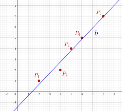
$$ \mathbf{\beta}_0 + \mathbf{\beta}_1\mathbf{x} = \begin{pmatrix} -1.45 + 1.05\cdot 2 \\ -1.45 + 1.05\cdot 4 \\ -1.45 + 1.05\cdot 5 \\ -1.45 + 1.05\cdot 6 \\ -1.45 + 1.05\cdot 8 \end{pmatrix} = \begin{pmatrix} 0.65 \\ 2.75 \\ 3.80 \\ 4.85 \\ 6.95 \end{pmatrix} \approx \begin{pmatrix} 1 \\ 2 \\ 4 \\ 5 \\ 7 \end{pmatrix} = \mathbf{y}. $$This is the "accuracy" of the simultaneous simple linear regression method. Image top left shows the n = 5 red points P1(2, 1), P2(4, 2), P3(5, 4), P4(6, 5) and P5(8, 7) of this example and the blue line b of the simultaneous linear regression.
3. Let's compare this result with what the least squares method would find. We calculate the mean values of the given sequences x = (2, 4, 5, 6, 8) and y = (1, 2, 4, 5, 7), which are μx = ∑ x/n = 25/5 = 5.0 and μy = ∑ y/n = 19/5 = 3.8, and form the joins and use them to form the correlation:
sx = x - μx = (-3, -1, 0, 1, 3), sy = y - μy = (-2.8, -1.8, 0.2, 1.2, 3.2), sx⋅sy = (-3)⋅(-2.8) + (-1)⋅(-1.8) + 0⋅0.2 + 1 ⋅1.2 + 3⋅3.2 = 21.0 κ(x, y) = sx⋅sy/[√(9 + 1 + 0 + 1 + 9)(7.83 + 3.24 + 0.04 + 1.44 + 10.24)], κ(x, y) = 21/(4.47⋅4.77), κ(x, y) = 0.98.
Least squares linear regression has the formula y = a + bx, where:
b = 0.98⋅4.77/4.47 = 1.05, a = 3.8 - 1.05⋅5 = -1.45
approximately. Thus we obtain the regression line using the least squares method:
y = -1.45 + 1.05 x
and that is the regression line using the simultaneous method, which we calculated previously.
4. Finally, let's look at an easy example of simultaneous multiple linear regression y = β0 + β1 x1 + β2 x2, with the sums in a table:
| y | x1 | x2 | x1y | x1² | x1x2 | x2y | x2² |
|---|---|---|---|---|---|---|---|
| 1 | 2 | 3 | 2 | 4 | 6 | 3 | 9 |
| 2 | 4 | 5 | 8 | 16 | 20 | 10 | 25 |
| 4 | 5 | 10 | 20 | 25 | 50 | 40 | 100 |
| 5 | 6 | 11 | 30 | 36 | 66 | 55 | 121 |
| 7 | 8 | 13 | 56 | 64 | 104 | 91 | 169 |
| 19 | 25 | 42 | 116 | 145 | 246 | 199 | 424 |
We need this because we multiply the linear regression equation by the first and then the second variable to obtain a system of three linear equations:
∑ y = n β0 + β1 ∑ x1 + β2 ∑ x2, ∑ x1y = β0 ∑ x1 + β1 ∑ x1² + β2 ∑ x1x2, ∑ x2y = β0 ∑ x2 + β1 ∑ x1x2 + β2 ∑ x2².
The sums (bottom of the table) give the linear equations of the unknowns β0, β1 and β2:
19 = 5 β0 + 25 β1 + 42 β2, 116 = 25 β0 + 145 β1 + 246 β2, 199 = 42 β0 + 246 β1 + 424 β2.
This is a linear system, α = M β, with a symmetric third-order matrix, which for the sake of simplicity we will now solve by elimination. We multiply the first of the three equations by -5, then add the result to the second; we mult-iply the first by -42/5, then add it to the third; we get:
21 = 20 β1 + 36 β2, 197 = 180 β1 + 356 β2.
This is a linear system of two equations. We multiply the first by -9, then add them, we get 8 = 32 β2 and hence:
β2 = 1/4 = 0.25.
Putting this back into the first previous equation, 21 = 20 β1 + 36/4, we find that 3 = 5 β1 and hence:
β1 = 3/5 = 0.6.
Let's put both found parameters back into the very first equation; we get:
19 = 5 β0 + 25⋅3/5 + 42/4, -13 = 10 β0, β0 = -13/10 = -1.3.
Accordingly, it is:
y = β0 + β1 x1 + β2 x2,
y = -1.3 + 0.6 x1 + 0.25 x2
The plane of the linear regression in the rectangular system yx1x2 which we found using the simultaneous method.
Coincident » srb
Question: What is the advantage of the "simultaneous" linear regression?
Answer: Simplicity, if that is an ad-vantage for statisticians and other users of these methods. This is, fi-rst of all, a benefit for the work of theorists, and possibly for some others, for example, to notice when this regression will not work. The previous answer is easy to genera-lize.
1. Let us now write the equation of the given multilinear regression in the form with small xs (they are usually large, with small ys) and introduce the m-tuple x0 = (1, 1, ..., 1) which does not exist otherwise:
y = β0x0 + β1x1 + ... + βnxn,
where the elements of the m-tuple xk = (ηjk) are real or complex numbers. Then we form systems of linear equations by scalar multiplications:
$$ \langle x_j|y\rangle = \sum_{k=0}^n \beta_k \langle x_j|x_k\rangle, \quad j = 0, 1, ..., n. $$The same written in matrix (α = M β) are:
$$ \begin{pmatrix} \langle x_0|y\rangle \\ \langle x_1|y\rangle \\ ... \\ \langle x_n|y\rangle \end{pmatrix} = \begin{pmatrix} \langle x_0|x_0\rangle & \langle x_0|x_1 \rangle & ... & \langle x_0|x_n\rangle \\ \langle x_1|x_0\rangle & \langle x_1|x_1 \rangle & ... & \langle x_1|x_n\rangle \\ ... & ... & ... & ... \\ \langle x_n|x_0\rangle & \langle x_n|x_1 \rangle & ... & \langle x_n|x_n\rangle \end{pmatrix} \begin{pmatrix} \beta_0 \\ \beta_1 \\ ... \\ \beta_n \end{pmatrix}, $$where all coefficients are known except the one on the right, the vector beta. To find the vector beta, we need a regular matrix M, which implies that its determinant det(M) ≠ 0, i.e. we can write β = M-1α. But this means that the vectors xk are linearly independent of each other.
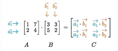
In the figure on the left, we see a simple example of a matrix, denot-ed C, of the dot products of vectors. It is obtained by multiplying two matrices, AB = C. In addition, it is known that the determinant of the product det(AB) is equal to (det A) (det B). Hence, the vectors xk are linearly independent iff det(M) ≠ 0.
2. In the previous answer (Simultaneous, 4) there was also a matrix (3 × 3) which is first in general form, with perhaps complex coefficients, where col-umn vectors are implied:
$$ X^\dagger X = M, $$ $$ \begin{pmatrix} x_0^\dagger \\ x_1^\dagger \\ x_2^\dagger \end{pmatrix} \begin{pmatrix} x_0 & x_1 & x_2 \end{pmatrix} = \begin{pmatrix} \langle x_0|x_0\rangle & \langle x_0|x_1\rangle & \langle x_0|x_2\rangle \\ \langle x_1|x_0\rangle & \langle x_1|x_1\rangle & \langle x_1|x_2\rangle \\ \langle x_2|x_0\rangle & \langle x_2|x_1\rangle & \langle x_2|x_2\rangle \end{pmatrix}, $$ $$ \begin{pmatrix} 1 & 1 & 1 & 1 & 1 \\ 2 & 4 & 5 & 6 & 8 \\ 3 & 5 & 10 & 11 & 13 \end{pmatrix} \begin{pmatrix} 1 & 2 & 3 \\ 1 & 4 & 5 \\ 1 & 5 & 10 \\ 1 & 6 & 11 \\ 1 & 8 & 13 \end{pmatrix} = \begin{pmatrix} 5 & 25 & 42 \\ 25 & 145 & 246 \\ 42 & 246 & 424 \end{pmatrix}. $$The matrices on the left are not square and do not have determinants, but their square matrix parts do and they are nonzero. The determinant of this matrix is det(M) = 640, and the inverse is:
$$ M^{-1} = \begin{pmatrix} 1.50625 & -0.41875 & 0.09375 \\ -0.41875 & 0.55625 & -0.28125 \\ 0.09375 & -0.28125 & 0.15625 \end{pmatrix} $$so from the linear system, $\vec{\alpha} = M\vec{\beta}$, knowing the alphas we find the betas:
$$ \vec{\beta} = M^{-1}\vec{\alpha}, $$ $$ \begin{pmatrix} \beta_0 \\ \beta_1 \\ \beta_2 \end{pmatrix} = \begin{pmatrix} 1.50625 & -0.41875 & 0.09375 \\ -0.41875 & 0.55625 & -0.28125 \\ 0.09375 & -0.28125 & 0.15625 \end{pmatrix} \begin{pmatrix} 19 \\ 116 \\ 199 \end{pmatrix}, $$ $$ \begin{pmatrix} \beta_0 \\ \beta_1 \\ \beta_2 \end{pmatrix} = \begin{pmatrix} -1.3 \\ 0.6 \\ 0.25 \end{pmatrix}, $$and the same, in another way, was obtained in the aforementioned answer.
3. Multiple linear regression is a way of saying, “We’re trying to predict so-mething based on a bunch of different factors.” For example, when making a smoothie (thicker fruit drink) each of the ingredients (banana, yogurt, honey) adds something to the final taste. Each Xk (for k = 1, 2, ..., n) as an indepen-dent variable, called a predictor, contributes to predicting the outcome, or dependent variable y = β0 + β1X1 + ... + βnXn. And every time we pour the same ingredients, say, making a smoothie, we expect to get the same taste of the drink — even though the ingredients are independent of each other. This is very important for understanding output expectations and input independe-nce.
4. The advantage of the simultaneous method is also seen in the case where every Hermitian (symmetric) matrix M has real eigenvalues λ ∈ ℝ and to wh-ich belong the eigenvectors $\vec{v}$ so that $M\vec{v} = \lambda\vec{v}$. If such an eigenvector happ-ens to be beta, $M\vec{\beta} = \lambda\vec{\beta}$, then $\lambda\vec{\beta} = \vec{\alpha}$, so all the coordinates of the vector alpha become scalar products of the independents with the dependent vari-able, $\vec{\alpha} = (\langle \vec{x}_k|\vec{y}\rangle)$ with k = 0, 1, ..., n. I put arrows above these m-tuples to emphasize their vector nature.
In other words, if it happens during the measurement of random outcomes $\vec{x}_k = (\xi_{jk})$, where ξjk ∈ ℂ with j = 1, 2, ..., m and k = 0, 1, ..., n, that they give exactly the eigenvector $\vec{\beta}$ of the matrix $M = (\langle x_j|x_k\rangle)$ of order n+1, then the elements $\langle \vec{x}_k|\vec{y}\rangle = \lambda\beta_k$ of the vector alpha will be projections of the indepen-dent random variables $\vec{x}_k$ onto the dependent variable $\vec{y}$. Regardless of whe-ther such a thing happens with a given measurement, the simultaneous meth-od reveals that possibility as always present, latent, and even the very logic of the aforementioned expectation (taste from independent additives).
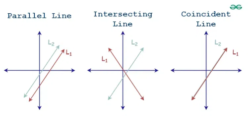
5. Coincidence (coexistence, simultaneity) in statistics has a somewhat dist-orted, shifted meaning compared to geometric (see image and link, up right). As in the dilemma of what came first, the chicken or the egg, in the informa-tion theory we are discussing, it is a question of the primacy of chance and causality. Consistently, I adhere to the priority of chance from which causality arises using reality (observable, sustainable, true) repetition and regularity of large numbers. Matrices like M and the processes described by them or simi-lar, also speak of local divergence and global convergence.
Least squares II » srb
Question: Where can I find a proof of the "least squares" method for multiple linear regression?
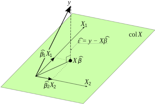
Answer: You can find out more ab-out it at the image link on the left. I believe it's better than what I can tell you right now. But, here you go, take your pick.
Common in the calculation of sim-ple or multiple linear regression is the initial formula:
y = β0 + β1X1 + ... + βnXn
where n = 1, 2, 3, ..., the vectors Xk = (ξ1k, ξ1k, ..., ξmk) are all m-tuples of nu-mbers to which I usually add only one more such X0 = (1, 1, ..., 1) for the sake of more convenient further writing.
1. Matrix, y = Xb, with vectors, one m-tuple y = (η1, η2, ..., ηm) and n+1-tuple b = (β0, β1, ..., βn), we write that:
$$ \begin{pmatrix} \eta_1 \\ \eta_2 \\ ... \\ \eta_m \end{pmatrix} = \begin{pmatrix} 1 & \xi_{11} & ... & \xi_{1n} \\ 1 & \xi_{21} & ... & \xi_{2n} \\ ... & ... & ... & ... \\ 1 & \xi_{m1} & ... & \xi_{mn} \end{pmatrix} \begin{pmatrix} \beta_0 \\ \beta_1 \\ ... \\ \beta_n \end{pmatrix}. $$We recognize this matrix from the equation $X^\dagger X = M$ of the previous answer (Coincident, 2). Otherwise, the adjoint of X† is the conjugation with the trans-pose of the matrix X, but in statistics that only uses real numbers it is just the transpose, X† = (X*)⊤ = X⊤. This is the initial form from the actual measurem-ent. The dependent variable given by the formula is $\hat{y} = (\hat{\eta}_1, \hat{\eta}_2, ..., \hat{\eta}_m)$, with the error e = y - ŷ also a vector, the m-tuple e = (ε1, ε2, ..., εm), so $\varepsilon_j = \eta_j - \hat{\eta}_j$ for each j = 1, 2, ..., m.
2. In the previous answer, we found one solution to multiple linear regression. It is based on the scalar products (arrays) of random variables, or their intern-al information (In and Out), while now we are looking for a solution for the minimum value of the sum of squares:
$$ E = \|e\|^2 = \langle e|e\rangle = (\eta_1 - \hat{\eta})^2 + (\eta_2 - \hat{\eta}_2)^2 + ... + (\eta_m - \hat{\eta}_m)^2. $$This "error function" is written in matrix form:
$$ E = e^\dagger e = (y - \hat{y})^\dagger (y - \hat{y}) = (y^\dagger - \hat{y}^\dagger)(y - \hat{y}) = $$ $$ = [y^\dagger - (Xb)^\dagger][y - (Xb)] = y^\dagger y - y^\dagger (Xb) - (Xb)^\dagger y + (Xb)^\dagger(Xb), $$ $$ Е = y^\dagger y - 2y^\dagger(Xb) + b^\dagger Mb. $$We have noticed that the last sumand (Xb)†(Xb) = b†X†Xb = b†Mb, where M is symmetric, it is also Hermitian M† = M, the matrix from the previous answer. In addition, the second and third summands are equal if they have real coeffi-cients, y†(Xb) = (Xb)†y.
3. The second and third summands of the real coefficients are equal. Namely, we can write this second summand in the form:
$$ y^\dagger(Xb) = \begin{pmatrix} \eta^*_1 & \eta^*_2 & \dots & \eta^*_m \end{pmatrix} \begin{pmatrix} \beta_0 + \xi_{11}\beta_1 + ... + \xi_{1n}\beta_n \\ \beta_0 + \xi_{21}\beta_1 + ... + \xi_{2n}\beta_n \\ \dots \\ \beta_0 + \xi_{m1}\beta_1 + ... + \xi_{mn}\beta_n \end{pmatrix} = $$ $$ = \beta_0\sum^m_{j=1} \eta^*_j + \beta_1\sum^m_{j=1} \eta^*_j \xi_{j1} + ... + \beta_n \sum^m_{j=1} \eta^*_j \xi_{jn} = \sum_{k=0}^n \sum_{j=1}^m \beta_k \eta_j^* \xi_{jk} $$ $$ y^\dagger(Xb) = \sum_{k=0}^n \beta_k \langle y | X_k \rangle. $$This is the second summation mentioned, and for the sake of brevity we have again (as in the previous answer) introduced the auxiliary sequence X0 = (1, 1, ..., 1) with m units. The third summation is:
$$ (Xb)^\dagger y = \begin{pmatrix} \beta_0 + \xi_{11}\beta_1 + ... + \xi_{1n}\beta_n \\ \beta_0 + \xi_{21}\beta_1 + ... + \xi_{2n}\beta_n \\ \dots \\ \beta_0 + \xi_{m1}\beta_1 + ... + \xi_{mn}\beta_n \end{pmatrix}^\dagger \begin{pmatrix} \eta_1 \\ \eta_2 \\ \dots \\ \eta_m \end{pmatrix} = $$ $$ = \beta^*_0 \sum^m_{j=1} \eta_j + \beta^*_1\sum^m_{j=1} \xi^*_{j1}\eta_j + ... + \beta^*_n\sum^m_{j=1} \xi^*_{jn}\eta_j = \sum_{k=0}^n\sum_{j=1}^n \beta_k^*\xi_{jk}^* \eta_j $$ $$ (Xb)^\dagger y = \sum_{k=0}^n \beta^*_k\langle X_k | y\rangle. $$However, if the coefficients are real numbers, then each $\beta^*_k = \beta_k$ and $\xi_{jk}^* = \xi_{jk}$ will also have each ⟨y|Xk⟩ = ⟨Xk|y⟩, so y†(Xb) = (Xb)†y.
4. While I'm already going into detail with this derivation, let's stop to prove the (well-known) theorem for matrix derivatives ∂x(x⊤Ax) = x⊤(A + A⊤), of the vector and matrix, i.e. x = (ξ1, ..., ξm)⊤ and A = (αjk), with indexes j = 1, 2, ..., m and k = 0, 1, ..., n, of the real coefficients. We have in order:
$$ f = x^\top Ax = \sum_{j=1}^m\sum_{k=0}^n \alpha_{jk}\xi_j\xi_k, $$ $$ \frac{\partial f}{\partial \xi_i} = \sum_{k=0}^n \alpha_{ik}\xi_k + \sum_{j=1}^m \alpha_{ji}\xi_j $$ $$ \frac{\partial f}{\partial x} = x^\top A^\top + x^\top A = x^\top (A^\top + A) $$and that's what we wanted to prove. Our coefficients (2) are real numbers. Our coefficients (2) are real numbers, so by finding the least sum of squares using the previous method, we find the derivative of the "error function" E and then set it equal to zero.
5. We seek the derivative of the sum of squares (E) to equalize it to zero and find the stationary point among which its minimum value is:
$$ \frac{\partial Е}{\partial b} = \frac{\partial}{\partial b}[y^\top y - 2y^\top(Xb) + b^\top Mb] = -2y^\top X + 2(X^\top X) b^\top = 0, $$ $$ (X^\top X)b^\top = y^\top X, $$ $$ b^\top = (y^\top X)(X^\top X)^{-1}, $$ $$ b = [(y^\top X)(X^\top X)^{-1}]^\top, $$ $$ b = [(X^\top X)^{-1}]^\top (y^\top X)^\top, $$ $$ b = (X^\top X^{-1})(X^\top y). $$It is the multiple linear regression formula with a proof that you will also find in the link above, here with explanations.
MLR Examples » srb
Question: Can you give me an example of solving this multi-linear regression formula (Least squares II, 5)?
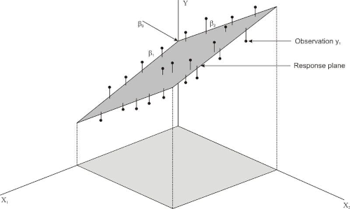
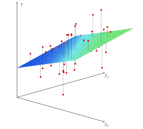
Answer: You can also find an exa-mple for testing at the image link on the right, and here I will show the actual use of that formula, b = (X⊤X-1)(X⊤y). Here b = (β0, β1, ..., βn), and the matrix X has units for the first column, then the column vectors X1, ..., Xn. Each are m-tu-ples of real numbers. When n = 2, we have a 3-dimensional space like the image on the right. The point Pj(ξj1, ξj2, ηj) has m, where j = 1, 2, ..., m. When n = 1 it is a 2-dimensional space. I will take as an example the first one from a recent answer (Simultaneous, 2), for easier learning.
1. Five-term arrays of random variables x1 = (2, 4, 5, 6, 8)⊤ and y = (1, 2, 4, 5, 7)⊤ were measured, which we will further treat as column vectors. Here n = 1 and in n+1 = 2-dim space we are looking for an equation line ŷ = β0x0 + β1x1 such that in the sense of "least squares" it best approximates the points (2, 1), (4, 2), (5, 4), (6, 5) and (8, 7) determined by them. We are looking for the vector "beta", b = (β0, β1)⊤, and we have added the vector x0 = (1, 1, 1, 1, 1,) to define the matrices X⊤X = M:
$$ \begin{pmatrix} 1 & 1 & 1 & 1 & 1 \\ 2 & 4 & 5 & 6 & 8 \end{pmatrix} \begin{pmatrix} 1 & 2 \\ 1 & 4 \\ 1 & 5 \\ 1 & 6 \\ 1 & 8 \end{pmatrix} = \begin{pmatrix} 5 & 25 \\ 25 & 145 \end{pmatrix} $$which we need to calculate the vector "beta" according to the "least squares" formula:
b = (X⊤X-1)(X⊤y) = [(X⊤X)-1]⊤(X⊤y) =
$$ = [(\begin{pmatrix} 1 & 1 & 1 & 1 & 1 \\ 2 & 4 & 5 & 6 & 8 \end{pmatrix} \begin{pmatrix} 1 & 2 \\ 1 & 4 \\ 1 & 5 \\ 1 & 6 \\ 1 & 8 \end{pmatrix})^{-1}]^\top (\begin{pmatrix} 1 & 1 & 1 & 1 & 1 \\ 2 & 4 & 5 & 6 & 8 \end{pmatrix} \begin{pmatrix} 1 \\ 2 \\ 4 \\ 5 \\ 7 \end{pmatrix}) $$ $$ = [\begin{pmatrix} 5 & 25 \\ 25 & 145 \end{pmatrix}^{-1}]^\top \begin{pmatrix} 19 \\ 116 \end{pmatrix} $$ $$ = \begin{pmatrix} 1.45 & -0.25 \\ -0.25 & 0.05 \end{pmatrix}^\top \begin{pmatrix} 19 \\ 116 \end{pmatrix} $$ $$ = \begin{pmatrix} 1.45 & -0.25 \\ -0.25 & 0.05 \end{pmatrix} \begin{pmatrix} 19 \\ 116 \end{pmatrix}, $$ $$ b = \begin{pmatrix} -1.45 \\ 1.05 \end{pmatrix} = \begin{pmatrix} \beta_0 \\ \beta_1 \end{pmatrix}. $$So, the best approximation of the given five points, this one by the method of "least squares", is the line ŷ = -1.45 + 1.05⋅x and it is the identical linear regr-ession that we obtained by working in a different way.
2. The second example is also from the aforementioned answer. Given random 5-tuples, independent variables x1 = (2, 4, 5, 6, 8)⊤ and x2 = (3, 5, 10, 11, 13)⊤ and dependent y = (1, 2, 4, 5, 7)⊤ with which we are looking for the line ŷ = β0x0 + β1x1 + β2x2 given the points (2, 3, 1), (4, 5, 2), (5, 10, 4), (6, 11, 5) and (8, 13, 7) are approximated by the least squares method. We find the vector b = (β0, β1, β2)⊤ by the above formula:
b = (X⊤X-1)(X⊤y) = [(X⊤X)-1]⊤(X⊤y) =
$$ = [(\begin{pmatrix} 1 & 1 & 1 & 1 & 1 \\ 2 & 4 & 5 & 6 & 8 \\ 3 & 5 & 10 & 11 & 13 \end{pmatrix} \begin{pmatrix} 1 & 2 & 3 \\ 1 & 4 & 5 \\ 1 & 5 & 10 \\ 1 & 6 & 11 \\ 1 & 8 & 13 \end{pmatrix})^{-1}]^\top (\begin{pmatrix} 1 & 1 & 1 & 1 & 1 \\ 2 & 4 & 5 & 6 & 8 \\ 3 & 5 & 10 & 11 & 13 \end{pmatrix} \begin{pmatrix} 1 \\ 2 \\ 4 \\ 5 \\ 7 \end{pmatrix}) $$ $$ = [\begin{pmatrix} 5 & 25 & 42 \\ 25 & 145 & 246 \\ 42 & 246 & 424 \end{pmatrix}^{-1}]^\top \begin{pmatrix} 19 \\ 116 \\ 199 \end{pmatrix}. $$The matrix M = X⊤X is symmetric, M⊤ = M. Its determinant is det M = 640, which means that it has an inverse matrix M-1, also symmetric, whose product with M is the identity matrix. Further:
$$ b = \begin{pmatrix} \beta_0 \\ \beta_1 \\ \beta_2 \end{pmatrix} = \begin{pmatrix} 1.50625 & -0.41875 & 0.09375 \\ -0.41875 & 0.55625 & -0.28125 \\ 0.09375 & -0.28125 & 0.15625 \end{pmatrix} \begin{pmatrix} 19 \\ 116 \\ 199 \end{pmatrix}, $$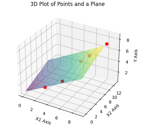
Again, the best approximation of the new spatial five points, with the "least squares" formula, is the line ŷ = -1.3 + 0.6⋅x1 + 0.25⋅x2 in the figure on the left. This is the mul-tiple-linear regression calculated earlier (Simultaneous, 4), when we found it in a different way. I hope the method is understandable (who asked me for it), but also how much the two do not differ in the end.
3. The following program (Python, 3.11.0) draws the previous graph:
import numpy as np
import matplotlib.pyplot as plt
from mpl_toolkits.mplot3d import Axes3D

# Equation ax + by + cz + d = 0 has normal vector [a, b, c]
normal = np.array([0.6, 0.25, -1])
# A point on the plane (e.g., when x1 = 0, x2 = 0, y = -1.3)
point = np.array([-1.3, 0, 0])
d = -point.dot(normal) # distance of the plane from O

# Create a grid for the plane surface
x1, x2 = np.meshgrid(range(10), range(10))
y = (-normal[0] * x1 - normal[1] * x2 - d) * 1. / normal[2]

# Define additional points to plot
points_to_plot = np.array([[2, 3, 1], [4, 5, 2], [5, 10, 4],
                           [6, 11, 5], [8, 13, 7]])

# Create the 3D plot
fig = plt.figure()
ax = fig.add_subplot(111, projection='3d')

# Plot the plane and points
ax.plot_surface(x1, x2, y, alpha=0.5, cmap='viridis')
ax.scatter(points_to_plot[:, 0], points_to_plot[:, 1],
           points_to_plot[:, 2], color='red', s=50)

# Set labels and title
ax.set_xlabel('X1 Axis')
ax.set_ylabel('X2 Axis')
ax.set_zlabel('Y Axis')
ax.set_title('3D Plot of Points and a Plane')

plt.show()
I usually keep these kinds of programs in modules, like Kodovi, with uniform inputs and outputs so they can be connected like Lego bricks.
4. This property of multiple linear regressions that they have widths, true dif-ferences that achieve the same thing, is fantastically instructive. For example, it is possible to have a given weight (y) if you are thin and tall (X1), or when you are fat and short (X2). It concerns the prevalence of abstract phenomena and stands in contrast to the uniqueness of concrete ones (Riesz Lemma). Th-at is actually a phenomenon that interests me more than these statistical cal-culations, but that is not the topic here.
Errors » srb
Question: How to evaluate the errors made by linear regression?
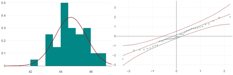
Answer: Let's take the previous examples to define the problem. First, there was a simple linear regression. It gave the points (x, y) ∈ (2, 1), (4, 2), (5, 4), (6, 5) and (8, 7) the ordinates ŷ(x) = -1.45 + 1.05⋅x. We calculate the ordinates point by point and subtract them from the given values:
ŷ(2) = 0.65 ŷ(4) = 2.75 ŷ(5) = 3.8 ŷ(6) = 4.85 ŷ(8) = 6.95; y(2) = 1 y(4) = 2 y(5) = 4 y(6) = 5 y(8) = 7; ε(2) = 0.35 ε(4) = -0.75 ε(5) = 0.2 ε(6) = 0.15 ε(8) = 0.05.
1. The errors ε(x) are small and uniform. The given points are close to the re-gression line and this is a good indicator of a normal distribution, which is a prerequisite for the application of this regression. Although the five given points are not enough for a good sample, they can be used for training.
2. Let's imagine that there are more random points and that their deviations from our estimate form a histogram (left part of the image above) that corres-ponds to the red bell curve of Gauss's (1809) normal distribution. That line is the graph of the probability density function:
$$ f(x) = \frac{1}{\sqrt{2\pi\sigma^2}}\exp\left(-\frac{x-\mu}{2\sigma^2}\right). $$The peak of the bell is above the abscissa of the expectation μ, in the case of many points with a mean error μ = 0, and the width of the bell is determined by the square root of the variance, or σ. In principle, a probability distribution is normal if the data are evenly, symmetrically distributed around a central mean. This is not the case for point estimate errors that follow a curved line.
3. Symmetries mean conservation laws. This was established among the first by Emmy Noether (Information Stories, p. 29), and we apply this here equally to the information (Physical Information, Theorem 2.4.16, p. 68) of the norm-al distribution SN = ln√(2πeσ²) and to the view that such a distribution has maximum information for a given dispersion (Extremes, 1.7). These three will discover an unofficial property of the normal distribution, that it takes on the maximum information (amount of uncertainty) and removes its superfluous presence from physical reality, in accordance with the principle of minimali-sm. I am talking about a part of (my) information theory that is not yet pres-ent in science, and therefore, which you can ignore.
4. I am writing this on 6 February, 2026, not so that you will believe it, but so that I may later refer to the following (hypo)thesis. Any rectilinear movement and abstract straight lines ultimately arise from the principle of minimalism and the aforementioned property of the normal distribution to absorb the maximum amount of information of a given variance σ². Then the measure-ment errors "left and right" of the estimated direction are approximately sym-metrically distributed. In fact, that is why they appear to be so, measured by physical means.
|
|
|