|
|
|


Coin flip » srb
Question: Can every random event be reduced to a 50/50 chance?

Answer: Interesting question, and that's why I included it in these an-swers. I know it was in some conv-ersation, but who knows when, in which one exactly, or on what occ-asion. There are at least two things that support a positive answer to this question: the reality of the case and its principled minimalism. But there is something else that makes this topic more interesting.
1. Reality does not like equality. I am paraphrasing one of the impor-tant consequences of the principle of minimalism, again, for the ump-teenth time, because it is still not part of official science.
For example, a fair coin, probability Pr("tails") = Pr("heads") = 1/2, has Shan-non information:
$$ S_1 = -\frac12\ln \frac12 - \frac12\ln \frac12 = \frac12\ln 2 + \frac12\ln 2 = \ln 2 \approx 0.69, $$while an unfair one, say with the probability Pr("tail") = 3/4 and Pr("head") = 1/4, would have such information:
$$ S_2 = -\frac34\ln \frac34 - \frac14\ln \frac14 \approx 0.56. $$In the second case, the “tail” is a more likely outcome and there is less news when it happens, so there is less uncertainty when tossing such an (unfair) coin and less information is brought to us by the realization of such an event. Nature spontaneously tends to more frequent realizations of more likely out-comes, less uncertain, and less informative, which means that the nature of reality also has a spontaneous tendency to less informative outcomes. This is the principle of minimalism. It then spontaneously leads reality in general towards the aforementioned inequality.
2. It is known that Shannon's information is a measure of the same amount of uncertainty before the realization as the information after. For example, the probability of the number "six" before rolling a fair die was 1/6, so this amou-nt of uncertainty is:
$$ S = -\frac16\ln\frac16 - ... - \frac16\ln\frac16 = 6\cdot(\frac16\ln 6) = \ln 6 \approx 1.79 $$and this is equal to the information of the outcome. Separately, it is equal to the Hartley information of such an outcome, $H = \ln 6$, six equal chances. This speaks of the maintenance of the amount of uncertainty during the realization itself, and even of the impossibility of realizing several such outcomes at once in reality, that is, permanent, observable and true events. However, we have no guarantee that such (fictitious) events will survive after or arise from noth-ing before the experiment. Moreover, we have lies that are just that: imperma-nent and unobservable to dead physical nature.
This is one of the reasons why we consider a particular time stream as the cu-rrent reality, without excluding the possibility of parallel similar pseudo-cur-rent streams, other dimensions of time. Whatever way such a reality, a given time stream of events, crystallizes, it has a problem with principled minimal-ism. Its information would like to disappear, but it must survive. It becomes, however, another reason for the thesis of an infinite (continuum, or larger) reservoir of possibilities sufficient to crystallize such a sustainability of our universe, which is its "problem".
3. The deepest uncertainty would be the one with equal chances, but we have seen that it is actually undesirable. On the other hand, we know that informa-tion from reality comes in packages. Hence the way of forming rational proba-bilities, of the form m/n, where m ∈ {0, 1, ..., n} and n ∈ ℕ, when we have a set of equally probable n, but in a package with such m. In addition, there are fu-rther uncountably infinite reservoirs of different possibilities, but not as phys-ical information, i.e. inaccessible to the measurements of classical physics.
4. Note that descriptions of "real" phenomena as perceptible, sustainable, and true do not exclude mathematical abstractions, and therefore "reality" cannot be limited only to what we can see, touch, or eat, but also to what (not everyt-hing) we can think about. In this sense, all random events can be reduced to half-and-half equal chances, real to rational numbers in the interval [0, 1] and hence to real in general.
Indicator II » srb
Question: Can the frequency of light be any real number and how, if possible, can I avoid this by calculating the frequency discretely?
Answer: In theory, the frequency of light (or electromagnetic radiation) is a continuum of quantities that can take on any positive real value, not limited to discrete sets of num-bers. Unlike the energies in an at-om, which are quantized, free pho-tons of the electromagnetic field take on continuous values of the frequency spectrum. I say restra-inedly, because there are ideas of limiting the duration to the Planck time tP ≈ 5.391×10-44 s (Graviton II). That is the time it takes for light with a speed of c ≈ 300 000 km/s to travel the distance ℓP ≈ 1.616×10⁻³⁵ m, one Planck length.
1. The frequencies of the visible light range from approximately 400 THz (red) to 790 THz (violet). These correspond to wavelengths from 750 to 380 nano-meters (nm). In this range, humans generally distinguish up to seven colors (violet, blue, cyan, green, yellow, orange, red), so we can distinguish about a million colors. But, it is estimated that, birds can perceive up to 100 million colors, because they are tetrachromatic. Bird eyes have four types of cone cells for colors (red, green, blue, and ultraviolet).
By the way, one tetrahertz (1 THz) has 1012 hertz (Hz), and one hertz is one cycle per second (s), so the range of light visible to us is approximately from 1.3×10⁻¹⁵ s to 2.5×10⁻¹⁵ s. In this range (1.2 ×10⁻¹⁵ s) there is room for more than 2×1028 Planck times. That is why even animals with the best vision do not perceive the possible discreteness of light frequencies, because it is neg-ligible even with the most accurate devices today.
2. Even without the (hypo)thesis of Planck time, it makes sense to approxim-ate the "discrete" frequency of light by a continuous one, because we often do something similar in reverse. For a start, try indicators. For example, let p ∈ (0, 1) be the probability that A will happen (falling a "head" when tossing a coin, falling a "six" when tossing a dice, etc.) and the probability q = 1 - p that A will not happen. Then the probability of event A, for the first time in the nth cycle, is Pn = qn-1p. The sequence P1, P2, P3, ..., is a well-defined probability dis-tribution, because it is determined by independent outcomes, is positive in number, and the sum of all is one.
3. I wrote about indicators in the book Physical Information (pp. 71-79) where you will find proofs of many interesting theorems, of which I will now mention only a few. The expectation of the number of attempts to the first desired eve-nt is μ1 = 1/p. The variance of the number of attempts of that distribution is σ1² = q/p². The Shannon information of such a distribution is:
$$ S_1 = -\sum_{k=0}^\infty P_k\ln P_k = -\sum_{k=0}^\infty q^kp\ln q^kp = $$ $$ = -\sum_{k=0}^\infty q^kp(k\ln q + \ln p) = -p\sum_{k=0}^\infty (kq^k\ln q + q^k \ln p) $$ $$ = -p \ln q \, \sum_{k=0}^\infty kq^k - p\ln p\,\sum_{k=0}^\infty q^k $$ $$ = -p\ln q\,\frac{q}{(1-q)^2} - p\ln p \, \frac{1}{1-q}, $$ $$ S_1 = \frac{1}{p}(-p\ln p - q\ln q). $$In that book, this is also physical information, L1 = S1, so called because of the undisguised conservation law that applies to it.
4. The probabilities of trying to reach the second desired event are:
P2 = p², P3 = 2p²q, P4 = 3p²q², ..., Pn = (n - 1)p²qn-2, ...
This is another well-defined probability distribution. The expectation of the number of trials of this distribution, the second desired event, is μ2 = 2/p = 2μ1, and the variance σ2² = 2q/p² = 2σ1². The physical information of the trials to the second desired event (L2), is distinguished from the Shannon (S2), and is:
$$ L_2 = -\sum_{n=2}^\infty (n-1)q^{n-2}p^2\ln q^{n-2}p^2 = ..., $$ $$ L_2 = \frac{2}{p}(-p\ln p - q\ln q), $$thus similar to the expectation and variance L2 = 2L1. The expectation, varia-nce, and physical information of the trials to the second desired outcome are twice as large as the corresponding trials to the first desired outcome. Unlike Shannon, Hartley's physical information (the logarithm of all of them) does not account for the variation in outcomes. Explicitly, these random events behave like fermions, and implicitly like bosons.
5. Let us now consider the repetition of a random experiment with a favorable outcome of constant probability 0 ≤ p ≤ 1 and an unfavorable outcome of pro-bability q = 1 − p until the favorable outcome occurs exactly m = 1, 2, 3, ... tim-es. With the repetition of the experiment n ∈ ℕ times and a favorable outcome 0 ≤ m ≤ n, the unfavorable outcome occurred n - m times. In the same book (Physical Information, 2019) with sometimes different labels, I provide details of the discussion and proofs of many positions, of which I only mention a few here.
An array of length n with m distinct elements but with one distinct element at the end of the array can be written on:
$$ \binom{n-1}{m-1} $$ways. Just like the same sequence without the last term, length n - 1 with m - 1 distincts. In each such sequence there are m favorable outcomes of probability p along with n - m unfavorable outcomes of probability q. It is of probability:
$$ P_n(m) = \binom{n-1}{m-1}p^mq^{n-m}, $$and the sum of all is Pm(m) + Pm+1(m) + Pm+2(m) + ... = 1, so these trials for any given m will form well-defined probability distributions. The expectation of such distributions is μm = m/p = mμ1, the variances are σm² = mq/p² = mσ1², with physical information:
$$ L_m = -\sum_{k=m}^\infty \binom{k-1}{m-1}q^{k-m}p^m\ln q^{k-m}p^m = ..., $$ $$ L_m = \frac{m}{p}(-p\ln p - q\ln q) = mL_1. $$This is the content of Theorem 2.5.13, of the above-mentioned book (p. 76), that the physical information of a distribution of “indicators m times” is exa-ctly m times the information of “indicators once”. In this case, the physical information is basically similar to Shannon’s, but in Hartley’s (logarithm of the number of equally probable) form without counting repeated combinati-ons and which we therefore treat as bosons.
6. I am listing all this only as one (probably unknown) model of a cycle such as a photon. For example, the number of repetitions m as the frequency, and the variance, or rather information, as a substitute for energy. That is the answer to the question. If that model were "too" good, compared to what it resembles, it would be "good enough" for physical reality. For that, we will put it through more difficult trials, but not this time.
Triangular II » srb
Question: I was attracted by the unusual analysis of the indicators. Have you also taken into account the variable probability indicators?
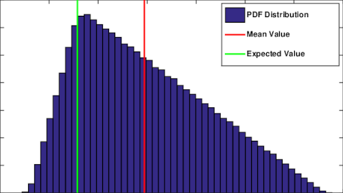
Answer: If you want to hear about a special kind of distribution, such as triangular, as a simpler type, I can explain it in the same way. The image on the left shows one such triangular probability distribution. They increase linearly from zero with the abscissa x = a, up to a maximum at x = c, and then decr-ease linearly to zero at x = b. Note that a < c < b. The blue surface of the triangle is colored by the ordinates ρ(x) of the probability density function (PDF) with the highest value along the green vertical line and the expected value along the red line.
1. With height h = 2/(b - a), the given triangle has vertices A(a, 0), B(b, 0) and C(c, 2/(b-a)) when it has unit area, and its upper edges thus define the proba-bility density ρ(x).The ordinates of the endpoints of the triangle are the proba-bility distribution densities:
$$ \rho(x) = \begin{cases} \frac{2(x-a)}{(b-a)(c-a)}, & x \in [a, c] \\ \frac{2(b-x)}{(b-a)(b-c)}, & x \in [c, b] \\ 0, & x \notin [a,b] \end{cases} $$Indeed:
$$ \int_0^b \rho(x)\,dx = \int_a^c \frac{2(x-a)}{(b-a)(c-a)}\,dx + \int_c^b\frac{2(b-x)}{(b-a)(b-c)}\,dx = $$ $$ = \frac{2(\frac{x^2}{2}-ax)}{(b-a)(c-a)} \Bigg|_a^c + \frac{2(bx-\frac{x^2}{2})}{(b-a)(b-c)}\Bigg|_c^b $$ $$ = \frac{2[\frac{c^2-a^2}{2}-a(c-a)]}{(b-a)(c-a)} + \frac{2[b(b-c)-\frac{b^2-c^2}{2}]}{(b-a)(b-c)} $$ $$ = \frac{c^2 - a^2 - 2ac + 2a^2}{(b-a)(c-a)} + \frac{2b^2 - 2bc - b^2 + c^2}{(b-a)(b-c)} $$ $$ = \frac{c^2 - 2ac + a^2}{(b-a)(c-a)} + \frac{b^2 - 2bc + c^2}{(b-a)(b-c)} $$ $$ = \frac{(c - a)^2}{(b-a)(c-a)} + \frac{(b-c)^2}{(b-a)(b-c)} $$ $$ = \frac{c-a}{b-a} + \frac{b-c}{b-a}, $$ $$ \int_0^b \rho(x)\,dx = 1. $$Therefore, the ordinates of the edges of a given triangle well define the density of the probability distribution. Triangular distributions defined in this way are often denoted by $\mathcal{T}(a,b,c)$.
2. You will find in the book Physical Information (Example 2.4.8, p. 60) a proof for the mathematical expectation of this distribution μ = (a + b + c)/3, and for the variance σ² = (a² + b² + c² - ab - bc - ca)/18. It is further easy to show that the upper green line is to the left of the red one, c < μ, whenever it is to the left of the middle of the base, c < (a + b)/2. The aforementioned book (previously this one) contains a description with some solutions of the com-plications that arise from breaking down the continuous triangular distribu-tion into discrete ones.
In short, we obtain a discrete triangular distribution when we divide the base b - a into, preferably more than, n equal parts, such that each part has length Δx = (b - a)/n. From the proportion n1 : n = (c - a) : (b - a) we get n1Δx = c - a, or the corresponding number of divisions n1 from the vertex A to the base of the altitude C1 of the triangle ABC, and then we calculate the probabilities, i.e. p(x) = ρ(x)Δx, that is:
$$ p(x) = \begin{cases} \frac{2(x-a)}{n(c-a)}, & x \in [a, c] \\ \frac{2(b-x)}{n(b-c)}, & x \in [c, b] \\ 0, & x \notin [a,b] \end{cases} $$Then we move on to the previous indicator calculation.
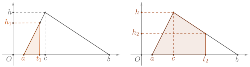
3. When we wait for the desired event with this probability, then the abscissa tells the time, t ∈ [a, b]. Before that (t ≤ a) the desired outcome certainly does not exist, while after that triangle (t ≥ c) the desired event certainly does. The chance that it will happen at the time of the triangle is:
$$ \Pr(x \le t) = P(t) = \int_a^t \rho(x)\,dx = \begin{cases} \frac12(t-a)h_1, & t \le c \\ 1 - \frac12(b-t)h_2, & t \ge c \end{cases} $$ $$ h_1 = \frac{2(t-a)}{(b-a)(c-a)}, \quad h = \frac{2}{b-a}, \quad h_2 = \frac{2(b-t)}{(b-a)(b-c)}. $$The explanation of these formulas is in the image above with two triangles. The probability that the desired event will occur is P(t) at time a ≤ t ≤ b. Bef-ore that it is zero, and after that it is one. If a given event were to repeat n = 1, 2, 3, ... times, with the same measured time, then Pm(t) is the probability that the desired event will occur m = 1, 2, ..., n times during that time and that it will not occur [1 - P(t)]n-m times. This is an analogous formula to the aforem-entioned discrete probabilities p(x). They lead to the same, but with much more complex explanations.
4. Multiply these two probabilities by the number of combinations $\binom{n-1}{m-1}$ so that in a sequence of n possible outcomes there are exactly m desired outco-mes. The last term of the sequence is certainly the desired one and we do not count it. Hence:
$$ \binom{n-1}{m-1}\,P^m(t)\,Q^{n-m}(t), \quad Q(t) = 1-P(t) $$is the probability that in n times of repeated chances, under the same conditi-ons of this triangular distribution, the desired outcome will occur exactly m times. The similarity with the corresponding result of the previous indicators is obvious. Hence the expectation that in n ∈ ℕ cycles fixed durations t ∈ [a, b] the desired outcome occur exactly m ∈ {1, 2, ..., n] times μm = mμ1 = m/P(t). Also the variance σm² = mσ1² = mQ(t)/P(t), and the physical information is:
$$ L_m = -\int_0^t\binom{n-1}{m-1}P^m(x)Q^{n-m}(x) \ln P^m(x)Q^{n-m}(x) \, dx = ..., $$ $$ L_m = \frac{m}{P(t)}[-P(t)\ln P(t) - Q(t)\ln Q(t)] = mL_1 $$and is m times greater than the information of the occurrence of one desired outcome.
5. The Shannon information of the triangular distribution (Physical Informati-on, Theorem 2.4.15, p. 66) is:
$$ S_\mathcal{T} = \ln \frac{(b-a)\sqrt{e}}{2}. $$Classical, or Shannon, is less than physical information because:
$$ \binom{n-1}{m-1} \gt 1, $$ $$ \binom{n-1}{m-1}P^m(x)Q^{n-m} \gt P^m(x)Q^{n-m}, $$ $$ [\binom{n-1}{m-1}P^m(x)Q^{n-m}]^{-1} \lt [P^m(x)Q^{n-m}]^{-1}, $$ $$ - \ln \binom{n-1}{m-1}P^m(x)Q^{n-m} \lt -\ln P^m(x)Q^{n-m}. $$Because the number of logarithms on the left is greater than on the right, it becomes $S_\mathcal{T} \lt L_m$, so the law of conservation of information applies to the physical one. I use this in distinguishing internal from external information (In and Out).
Performances » srb
Question: Explain to me a little "inside" information, if that's possible without formulas?

Answer: What you are asking for is possible. Verification by formulas strengthens the statement so that it proves to be true in every exact fra-mework, in mathematics, and only then can intuition act almost as fl-awlessly. Only theorems are the foundation for unlimited series of deductions, otherwise we quickly slide towards shallows, untruths. That is why we need formulas, but once we have them, it is easier to fantasize.
1. This also served as an introduction to the unique characteristics of the con-crete (Riesz Lemma) as opposed to the universality of the abstract. Subjects, living or non-living, perceive the world around them in unique ways; no two such couplings (two pieces of perceptual information) are exactly the same, not even in the same subject at two different moments. This already tells us about something "inside", which we do not see. With vitality itself, which is an addition to inanimate physical things, we have the power to fantasize and lie. This is what a non-vital physical substance cannot do, and which is also a “cu-rse” that add-itionally burdens us with its untruths. With vitality, “internal” information both moves away from us and closer to us. I will explain the latter as well.
2. When we statistically analyze the communication of dolphins, or the chirps of birds (a magpie's long "kraaa" means "friend," while a short "kra-kra" mea-ns "danger"), we discover more order than would be expected spontaneously. Likewise in the choice of chemicals by which ants communicate, or the scents of animals with a sense of smell. Fireflies (Latin: Lampyridae) are insects of the genus Lampyridae, named for their ability to glow at night to attract mates or prey, and their choice of signals to be more specific. Light also appears in its colors, but a deeper meaning gives them vitality.
Analysis of the letter frequency of meaningful text shows lower information content than nonsense. This fall reveals to us a possible communication, be-fore we even know who they are or what these creatures would be talking ab-out. In other words, intelligence gives us momentum, like the potential of a raised pickaxe, to dive below the normal level of uncertainty of the inanimate world. That lower world is the world of rules, logic and deeper meaning, say, of scientific order or the mastery of inherent intelligences. In this way, we also dive to “inner” information.
3. Natural phenomena communicate; in physics, we mean interact. Each of the participants, individually, according to their capabilities and in their own way, addresses the environment, presents themselves, and fails to expose their entire "essence," because it does not actually exist in the way we usually imagi-ne it, even when they give themselves over completely. The representation of the external information of each natural phenomenon is never an accurate re-presentation of its interior, otherwise there would be neither the mentioned uniqueness (Information Coupling, p. 124) nor the consequences, the inevita-ble diversity of the concrete (the same book, p. 127).
Hence the agreement between the addition of indicators (Indicator II, 5) and the superposition of waves, as well as some additive natural phenomena. On the other hand, we know that wavelengths exhibit uncertainties in the position of the flicker on their path, and that with them the Uncertainty Force that they covertly contain grows. This uncertainty is the internal power of fluttering that is more difficult to manifest, which is why pulses of longer wavelengths have a longer range and are longer-lived, are less consumed by the environment, and interact less with the surroundings, in informatic terms we would say they co-mmunicate less.
4. When we flip a coin twice, or flip two coins at once, we always know which is which in the sense that we have four independent outcomes {HH, HT, TH, TT}, landing “heads” and “tails”. Repeating this with fair coins, each of these four pairs will cluster around a quarter of the total tosses, and they would be a third when HT = TH. This is the fundamental difference between fermions, and here we would say actual coins or possibly external information, and bo-sons, internal information. These internal ones seem to pack themselves into smaller ones while pretending they don't exist.
Coin flip II » srb
Question: Explain this last one to me, coin tossing (4), if possible as simply as "performance", so that I can better understand the difference between physic-al and classical information?
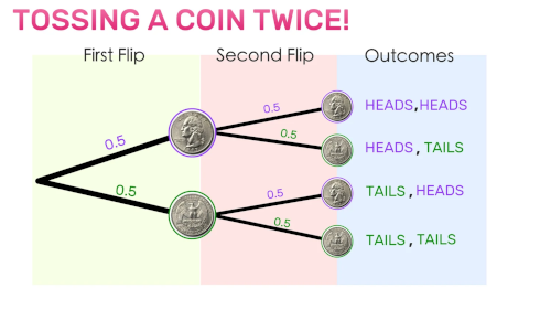
Answer: Okay. Let's go in order. We first flip just one coin, then two, then three, to see the changes in ex-pectations, variances, then Shann-on information and these new, so-called physical ones.
1. If we toss only one coin (fair), th-ere are two equally likely outcomes ("tails" and "heads"). If we count the number of "heads" then x(T) = x0 = 0 and x(H) = x1 = 1. These notations should simplify the writing. The probabilities, expectation, and variance are:
$$ p_1(0) = \Pr(x_0) = \frac12, \quad p_1(1) = \Pr(x_1) = \frac12 $$ $$ \mu_1 = 0\cdot p_1(0) + 1\cdot p_1(1) = \frac12 $$ $$ \sigma_1^2 = (0 - \mu_1)^2\cdot p_1(0) + (1 - \mu_1)^2\cdot p_1(1) = 0.25 $$The most likely, mathematical expectation, is μ1 ± σ1, or 0.5 ± 0.5, which is from 0 to 1, which is not news. Shannon's information is:
$$ S_1 = -p_1(0)\ln p_1(0) - p_1(1)\ln p_1(1) = \ln 2 \approx 0.693 $$and that's the physical information of this one coin toss, L1 = S1. The differen-ce between the two appears when tossing two or more coins.
2. When we toss two coins, there are four possible outcomes TT, TH, HT, HH with each probability 1/4, but the number of "heads" has only three possibili-ties:
0: TT; 1: TH, HT; 2: HH
with probabilities, expectation, and variance:
$$ p_2(0) = \frac14, \quad p_2(1) = \frac12, \quad p_2(2) = \frac14 $$ $$ \mu_2 = 0\cdot p_2(0) + 1\cdot p_2(1) + 2\cdot p_2(2) = 1 $$ $$ \sigma_2^2 = (0 - \mu_2)^2\cdot p_2(0) + (1 - \mu_2)^2\cdot p_2(1) + (2 - \mu_2)^2\cdot p_2(2) = \frac12 $$Now the most likely, mathematical expectation, is μ2 ± σ2, or 1 ± 0.5, which is the number of "heads" from 0.5 to 1.5 in two attempts. Shannon's information is:
$$ S_2 = -\frac14\ln\frac14 - \frac12\ln\frac12 - \frac14\ln\frac14 = \frac32\ln 2 \approx 1.040 $$but the physical information (of tossing two coins) is:
$$ L_2 = -\frac14\ln\frac14 - \frac12\ln\frac12 - \frac14\ln\frac14 = 2\ln 2 = 2L_1 \approx 1.386. $$This is exactly twice the information of flipping a coin. What is happening here, I explained by the transformation of fermion-like behavior (coin dis-tinction) into boson-like behavior (non-distinction) and only for the Hartley information (logarithm of the number of equal outcomes) of that part of the phenomenon that becomes internal.
3. A third example, when we toss three fair coins and record how many times "heads" next to "tails" come up, all possible outcomes are:
0: TTT, 1: TTH, THT, HTT 2: THH, HTH, HHT 3: HHH
When we plot these sums, from 0 to 3, along the abscissa, we get a triangular distribution graph. There are eight outcomes in total, so we have the (only non-zero) probabilities, then the expectation and the variance:
p3(0) = 1/8, p3(1) = 3/8, p3(2) = 3/8, p3(3) = 1/8
$$ \mu_3 = \sum_{k=0}^3 k\cdot p_3(k) = \frac32 $$ $$ \sigma_2^2 = \sum_{k=0}^3 (k-\mu_3)^2\cdot p_3(k) = \frac34 $$This mathematical expectation (μ3 = 1.5) tells us what the most likely outcome is in tossing three coins, that one and a half heads will come up. The variance (expected squared deviation from the expectation) of such an experiment is σ3² = 0.75 and this tells us about the width, the range of these most likely ou-tcomes, from μ3 - σ3 to μ3 + σ3, or from 0.63 to 2.37. The information accordi-ng to Shannon would be:
$$ S_3 = -\sum_{k=0}^3 p_3(k) \ln p_3(k) \approx 1.255 $$while physical information is:
$$ L_3 = -\sum_{k=0}^3 p_3(k)\ln\frac18 = 3\ln 2 = 3L_1 \approx 2.079. $$In tossing three coins, the physical information is exactly three times the info-rmation in tossing one coin. The fact that all these results agree so precisely is an important argument in favor of the accuracy of this part of the theory.
4. In all such further cases, of tossing m = 2, 3, 4, ... coins, the Shannon infor-mation will be less than the physical one (Sm < Lm), and the physical one is m times the physical one of tossing one coin (Lm = mL1). I have given it the name "physical information" because it completely imitates the law of conservation (of information) and because it well describes some natural phenomena that I have mentioned more often before.
Continuing the course here, we also notice the simulation of principled mini-malism using physical information, in the sense that complex phenomena co-nceal their excess information when they can no longer get rid of it. Secondly, this is how excess uncertainty is kept separate, inactive by external represen-tations, which is why the phenomenon actually survives in the sense of this theory where information makes up the fabric of space, time and matter, and uncertainty is its essence.
Binomial II » srb
Question: Does your story about "physical information" also apply to flipping an unfair coin many times?
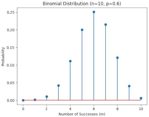
Answer: Yes, I'll explain, and you decide for yourself. First, a brief introduction to the binomial dis-tribution, fundamental to proba-bility theory and so to statistics. The Binomial distribution is also topic in theory of information.
1. A single coin flip will resolve the dilemma of two choices, "tails" and "heads". It is similar to the binary digits 0 and 1 competing for the same position. Double places, the two positions contain four (2²) different binary numbers: 00, 01, 10, 11. These are the decimal numbers: 0, 1, 2, 3. Three places have the capacity for eight (2³) different binary numbers: 000, 001, 010, 011, 100, 101, 110, 111. These are the eight numbers from zero to seven, inclusive. In general, if three positions are added to two positions, five positions are obtained (2²⋅2³ = 22+3), and if an n-m position is added to some m ∈ ℕ positions, (0 ≤ m ≤ n ∈ ℕ), the n position is obtained, 2m⋅2n-m = 2m+(n-m) = 2n. This kind of additivity is transferred to Hartley's information.
2. When the occurrence of the digits 0 and 1 in positions is equal, then the nu-mber n positions is the Hartley information of the number 2n possible recor-ds. The inverse is also true. If we have N ∈ ℕ equally likely possibilities, then the Hartley information will be equal to the logarithm of the base two of that number, log2N bits (BInary digiT). Thus, Hartley information is "physical", unlike Shannon information.
Although N = 1, 2, 3, ... is a natural number, its logarithm is not, so when we have a positive real number, r ∈ ℝ+, we approximate it, divide it into approxi-mately equal parts, and declare logb r to be the same Hartley information. Th-is is again additive, therefore "physical", because combining N1 possibilities with N2 options gives N1⋅N2 options, and logb(N1⋅N2) = logb(N1) + logb(N2). The base of the logarithm (b > 0) defines the base, in physics we say the dim-ension, the size of the information.
3. Let's imagine further that we have some unfair lotto machine that generates the number 1 with probability p = 0.6 and the number 0 with probability q = 1 - p = 0.4. For example, if in a series of n = 10 draws there were m = 3 ones, th-en there were n - m = 7 zeros in that series. Each one had probability p = 0.6 and each zero had probability q = 0.4, so one such series had probabilities:
pm⋅qn-m = p3⋅q7 = 0,63⋅0,47 ≈ 0.00035
from which we estimate that this is only a small number of the many other arrangements in the same 10 draws. This is just one possibility out of all the combinations:
$$ \binom{n}{m} = \frac{n\cdot(n-1)\cdots(n-m+1)}{1\cdot 2 \cdots m} = \frac{10\cdot 9\cdot 8}{1\cdot 2\cdot 3} = 120. $$When we add them all up, we find:
$$ \sum_{m=0}^n \binom{n}{m}p^mq^{n-m} = (p + q)^n = 1, $$whenever p + q = 1, then we have a well-defined probability distribution of numerous independent outcomes, some of which are certain to occur.
4. In the image above on the right is the binomial distribution:
import numpy as np
import matplotlib.pyplot as plt
from scipy.stats import binom

n, p = 10, 0.6
m = np.arange(0, n + 1)
pr = binom.pmf(m, n, p)
print(f"The probability {m} successes in {n} trials: {pr}")

plt.stem(m, pr)
plt.title(f'Binomial Distribution (n={n}, p={p})')
plt.xlabel('Number of Successes (m)')
plt.ylabel('Probability')
plt.show()
It is a Python program that will display the following text in addition to the image on the screen:
The probability [ 0  1  2  3  4  5  6  7  8  9 10] successes
in 10 trials: [1.04857600e-04 1.57286400e-03 1.06168320e-02
	       4.24673280e-02 1.11476736e-01 2.00658125e-01
	       2.50822656e-01 2.14990848e-01 1.20932352e-01
	       4.03107840e-02 6.04661760e-03]
where the fourth of these numbers is the upper probability and multiplied by its binomial coefficient $\binom{10}{3}\cdot 0.6^3 \cdot 0.4^7 \approx 0.042467$. The figure shows all 11 options, the points above the abscissa with the number of desired outcomes and the ordinates with the binomial probabilities.
5. If we remove the binomial coefficient $\binom{n}{m}$ and keep only the product of pro-babilities $p^mq^{n-m}$, simply put, we move from fermions, i.e. Fermi-Dirac stati-stics:
$$ f_F(\varepsilon) = \frac{1}{e^{(\varepsilon - \mu)/kT} + 1} $$on the so-called bosons, or Bose-Einstein statistics:
$$ f_B(\varepsilon) = \frac{1}{e^{(\varepsilon - \mu)/kT} - 1} $$where, in quantum physics, ε is the energy of the state, μ is the chemical pote-ntial, k is the Boltzmann constant, and T is the absolute temperature. These functions f(ε) are the average values of the number of particles of energy ε under given conditions, chemical environment, and temperature. A smaller denominator gives a larger number fB for the same environment.
Unlike Bose–Einstein statistics, which applies to particles of integer spin (bos-ons), Fermi–Dirac statistics, which applies to particles of half-integer spin (fe-rmions), restricts them to those that identical cannot be in the same state, so reducing their number and narrowing their choices. Bosons therefore have a greater capacity for information, and thus the ability to absorb more uncerta-inty.
6. I gave the proof that the physical information (Ln) of the binomial distribut-ion ℬ(n, p) is worth n of the physical information (L1) of the unitary binomial distribution ℬ(1, p) in 2019 in the book Physical Information (Theorem 2.3.6, p. 50). You also have special examples there, proofs L2 = 2L1 and L3 = 3L1 for easier understanding of the general proposition. There is no need to rewrite them here.
Bounds » srb
Question: Can you give me a specific example of "physical information"?
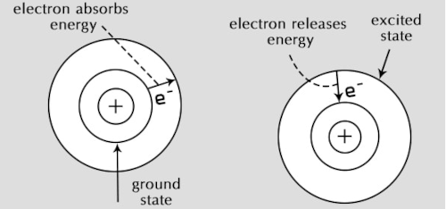
Answer: Hardly, experiments and that kind of science are not my do-main, so I can only fantasize. The link in the picture on the left has an explored yet inspiring interpretati-on of the transitions of electrons fr-om a higher to a lower shell of an atom when a photon is emitted and vice versa, the electron goes from a lower to a higher orbit when that energy is returned to it. Try in general, in the changes of potential, to find that "internal" accumulation. The correct theory, if "physical information" is what it is, will fit into this or that, in advance who knows how. Let's just remember Dirac's "playing" (in his words) with formulas (Spin III) which later proved practical.
1. Follow reality, speak the truth, but your greatest strength is in the unspok-en. This is a description of a character (Traits) that wins in the long run, consi-stent with the strategies of the first league of this theory, and in which we also recognize the concept of "physical information". A liar is disgusting when his broken promises are revealed, because he stinks of failure, of the builder of a house of cards, with which nature protects us through evolution as from the smell of rot, of plague, infectious diseases and ruin in general. Generations thus transmit fears of failure, aversion to the unsuccessful. However, in the short term, lying is attractive, sending us shallow truths that are underneath in contradictions and so convenient for "trick and run" tactics. A lie is a good pose for the outside world and a characteristic of impermanent phenomena.
In addition to duration and consistency (Packages III), which are more diffi-cult to measure characteristics of truth, its absence in complex phenomena can be recognized by popularity, the aforementioned property of lies. The appeal of lies in bacteria is seen in their ability to evade immune systems; for example, bacteria sometimes hide inside host cells to avoid detection. Or, de-spite their lack of a nervous system, many plants are very deceptive. This is the case, for example, with the bee orchid, which produces scents and shapes that imitate female insects, luring males to try to mate with them for the sake of its pollination. Lies are attractive and immediate, which is widely used by politicians in campaigning or salespeople in sales when deceiving the people, but also by artists simply to entertain their audience.
2. Physics is more rigorous than other sciences, it is more exact and more sui-table for testing new ideas if we seek their high accuracy, so we are required to compare “physical information” with a photon. The energy of a photon E = hf is proportional to the frequency f = 1/τ, where τ is the time of one period, one oscillation, and that's all, because h = 6.62607015 × 10⁻³⁴ m2 kg / s is the uni-versal Planck constant. Photons are bosons, so there is no described “conver-sion” of fermions into bosons.
When we compare the frequencies of light with indicators and repeat the exp-eriment, say with a variance σm² = mq/p² = mσ1² until the desired outcome occurs exactly m times, we should know that the uncertainties are not in the energy itself, but are packaged in the physical action, in the product of the change in energy (E) over the elapsed time (τ). However, that action, Planck's constant, does not change.
For example, this means that white light is a combination of different colors that exist as individual lights, as separate quanta, in that whole. The physical information of the whole, Lm = mL1, can then be a simple sum of internal in-formation. Applied to light sources in relative motion, this reveals interesting details.
3. In relative motion, the load of quanta do not change if we calculate them through the transverse relativistic Doppler effect. This is compared with the increase in energy, where v is the relative velocity, and c is the speed of light:
$$ f_T = \frac{f_0}{\sqrt{1 - \frac{v^2}{c^2}}}, \quad E_T = \frac{E_0}{\sqrt{1 - \frac{v^2}{c^2}}}, $$gives the unchanged Planck constant, h = ET/fT = E0/f0. However, there is a catch. The time of a body in relative motion is slowed down compared to its proper. We perceive its proper events as muffled, rarefied, with a smaller “amount of uncertainty” (information) and as confirmation of the “internal” accumulation of physical information. Otherwise, apart from the story with indicators, I interpret this slowing down as the departure of part of the inh-erent events into pseudo-reality, into additional dimensions of time. In its own way, this fits into “physical information” and even into the described preservation by transitioning to bosons.
Namely, what is real is that which has duration, has a past, and space is one of the repositories of the memory of reality. What we perceive in the distance is old and in that sense space-time is a complete concept whose structure is pri-marily made up of bosons. Therefore, the extraction of these arms of the syst-em in relative motion is made difficult by inertia, and then by the conversion of their potential energy into kinetic energy.
4. Energy is also spent on pulling a body out of a gravitational field, and it is assumed that this is a similar mechanism to inertial motion. I am thinking of the inverse model (2), which should then be verified by the theory of gravity (general relativity). Lifting a body, moving away from the center of the field, requires additional energy, and such a process is the inverse of the return of excess (kinetic) energy by stopping the body from its previous inertial motion. The quantum is of constant value (if it is), so for such two models the common attraction of the slower flow of time remains, and this is one detail of Einste-in's interpretation of gravity.
In combination with the above (2), the gravitational potential also makes it difficult to extract it from other dimensions of time of a given body. However, both models have the same cause (the principle of minimalism) - events spo-ntaneously flow towards more certain ones. Here we are left with two more questions, what about the potential of electrons in an atom and what about the potential of two electrons that repel each other.
Decay » srb
Question: Does the descent of electrons to lower atomic shells and the release of photons remind you of particle decays?
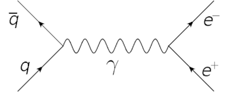
Answer: There are elements. The decay and fusion of particles via photons, as in the image on the left with the interpretation, indicates the connection mentioned in the question. It is also a reminder of how little we know about quantum physics. How many doors there are still waiting to be opened.
1. Due to the law of conservation of momentum and energy, a photon must interact with a strong electromagnetic field in order to decay into an electron and a positron, and in doing so, it must have an energy of at least 1.022 MeV, which is the total rest energy of the two particles into which it decays. The en-ergy of 1.022 MeV = 1.022 × 10⁶ eV corresponds to a frequency f ≈ 2.47 × 10²⁰ Hz, because Planck's constant h ≈ 4.1357 × 10⁻¹⁵ eV⋅s and E = hf. It correspon-ds to a wavelength λ ≈ 1.21×10⁻¹² m, and it belongs to the gamma rays.
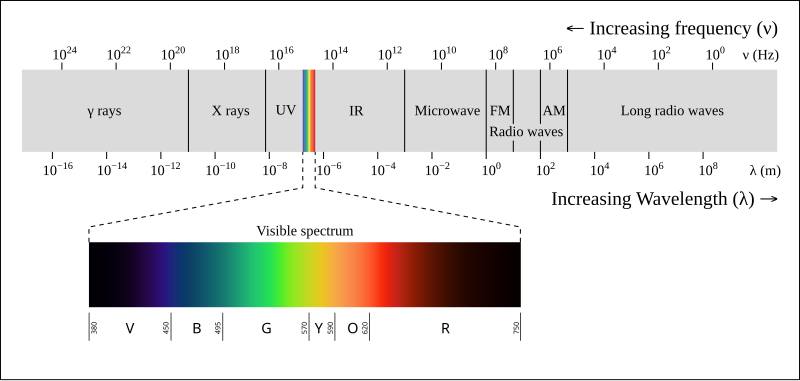
In the image above we see the entire light spectrum, with gamma rays to the left of the visible light portion. Therefore, it is possible, but not easy, for a ph-oton to decay into an electron and a positron. The walking of electrons throu-gh the shells of atoms, with the capture or release of corresponding photons, partly resembles the possibility of this decay.
2. Electrons and positrons are thus shown to be the structures of photons. Th-is is due to their reality (the law of conservation), and then due to the packagi-ng of information in quanta, the movement of electrons (negatively charged) from the nucleus of the atom (positively charged), indicates the same structu-re and charge of the atom itself. By emitting photons, by steps from higher to lower shells, this "indivisible" charge of electrons is decomposed by about -1.602 × 10⁻¹⁹ C (Coulomb).
On the other hand, it indicates the complexity of the composition of the infor-mation in the photon and its decomposition into energies and periods, or fre-quencies. Hence, again, we can compare them with the repetition of experim-ents until a given number of favorable outcomes is filled (Indicator II, 5). As the electron moves away from the nucleus, the opposite charges become ind-ependent, and this happens by replenishing photon quanta. I emphasize qua-nta, not energy (which is also correct), to emphasize the informational chara-cter of the process. Consistent with the principle of minimalism, we find that the electron spontaneously goes to lower orbitals, because then it is in less uncertainty.
3. If it is said well, then we are on the trail of explaining the quantization of li-ght in an atom as opposed to free photons. Some methods are already known, for example, the methods of annihilation and creation operators (Quantum Mechanics, Oscillator operators, p. 344), but here we deepen them by under-standing that information circulates through reality in packets, which are also found in light quanta. Their parts may be unreal, but still true abstractions and in abundance, even constantly present in unrelated places, unlike concre-te phenomena that are always different in relation to their environment (Riesz Lemma). The higher level of such packages are bosons, and further down in reality there are fermions.
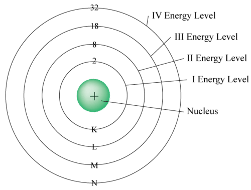
The leading (hypo)thesis of such an idea is the "cancellation" of opposi-te charges by bringing negative el-ectrons closer to the oppositely ch-arged nucleus of the atom. In the picture on the right, there are four electron shells in an atom where th-ey can have energies, the so-called series: Lyman, Balmer, Paschen, Brackett, and so on, with up to 2, 8, 18, 32, and even further electrons. Moving away from the nucleus, the energy of the electron also increas-es as the number of quanta, its packets of information, increases. Now we say that the electron resists this increase due to the principle of minimalism.
4. The maximum number of electrons per shell, from the bottom (ground sta-te) and up n = 1, 2, 3, ..., is 2n². The shells are divided into subshells (s, p, d, f) which contain orbitals, each with at most two electrons. The first shell (for n = 1) has one orbital (1s) with two electrons. The second shell (n = 2) goes up to four orbitals (2s, 2p) and eight electrons. The third shell (n = 3) also has nine orbitals (3s, 3p, 3d) with 18 electrons. The fourth (n = 4) has 16 orbitals (4s, 4p, 4d, 4f) with up to 32 electrons. The electrons in the outermost shell are known as valence electrons and are responsible for chemical bonding, while those closer to the atom already have enough information.
Orbitals » srb
Question: The interaction of a photon with an electron in an atom is also an interaction with the atom as a whole?
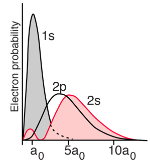
Answer: It can also be said that way, in a broader sense. The prin-cpal quantum number n = 1, 2, 3, ... tells us about the energy level of the electron (about 1 eV to 10³ eV):
$$ E_n = -hcR_\infty \frac{Z^2}{n^2}, $$where h is Planck's constant, c is the speed of light, R∞ is the Rydbe-rg constant, Z is the atomic number which indicates the atom's place in the periodic table, or the number of protons in the nucleus of an atom. The Rydberg formula is from:
$$ \frac{1}{\lambda} = R Z^2\left(\frac{1}{n_1^2} - \frac{1}{n_2^2}\right) $$combined with E = hf = hc/λ and the principal quantum number n = n1, and n2 → ∞. For example, the energies of bound electron states in a hydrogen at-om are also reduced to En = E1/n² = -13.6 eV/n². These notations are taken from the Bohr model. Mutual interactions of electrons increase the energy level, so the exact formulas are much more complicated, but we understand that even such roughly described energy levels of electrons are the main, the backbone of the further story about the atom. I'll explain in order.
1. An orbital is the most likely location of an electron in an atom. Increasing principal quantum number n = 1, 2, 3, ... means increasing electron energy, moving the most likely positions away from the nucleus, but also determines the shapes of those positions. The second quantum number ℓ ∈ {0, 1, ..., n-1} tells about the shape of the orbital. When ℓ = 0, the orbital is spherical and has the symbol s. The orbital at ℓ = 1 is labeled p and its shape resembles the sign ∞. When ℓ = 3, the orbital is labeled d and reminds us of a butterfly, and ℓ = 4 the orbital is labeled f with even more complex shapes.
The s symbol also means a sublevel of an orbital. Since ℓ is always ≤ n-1, the sublevel of the first level (n = 1) can only be ℓ = 0, which is an s orbital. The second level (n = 2) has orbitals: s for ℓ = 0 and p for ℓ = 1. Then the third level (n = 3) has orbitals: s for ℓ = 0, then p for ℓ = 1 and d for ℓ = 2. The fourth level (n = 4) has orbitals: s for ℓ = 0, p for ℓ = 1 and d for ℓ = 2. = 1, then d for ℓ = 2 and f for ℓ = 3. So, the first energy level has only 1s, while the second has two orbitals 2s and 2p, the third has 3s, 3p and 3d, and the fourth 4s, 4p, 4d and 4f. We also use these notations with chemical elements.
2. We notice that with increasing electron energy level, the forms (possibiliti-es) where the electron can be found in the atom increase step by step. This is also seen with the increase in magnetic quantum number mℓ ∈ {-ℓ, ..., ℓ} which is the third quantum number and it tells us about orientation. The sublevel s because of ℓ = 0 has only one position and one magnetic number mℓ = 0. With ℓ = 1 the sublevel p has three positions px, py and pz for orientations, extendi-ng the three magnetic numbers mℓ ∈ {-1, 0, 1}, in the form of the ∞ sign along the three coordinate axes.
The d sublevel goes with the second quantum number ℓ = 2 and has five orbit-als, with the third quantum number being the magnetic quantum numbers mℓ ∈ {-2, -1, 0, 1, 2}. The last, fourth quantum number is the electron spin, ms, which can have only two values, the so-called spin-up and spin-down. We say that they are clockwise and counterclockwise, or ms ∈ {+1/2, -1/2}. We also write the spin of electrons in an atom with an up arrow ↑ and a down arrow ↓.
3. The Pauli exclusion principle, proposed in 1925, states that no two electrons (or other fermions) in an atom or molecule can occupy the same quantum st-ate at the same time. Specifically, an atom has no two electrons with the same set of four quantum numbers n, ℓ, mℓ, and ms. In principle, an orbital can hold up to two electrons, then of opposite spins. Thus, the positions are filled, first with the same spin (it doesn't matter which one), and when doubling occurs, an electron of opposite spin is added.
Thus, the address 2p5 electrons means the second energy level n = 2, which means the sublevel ℓ = 1 and the p orbital, with mℓ in three sites {-1, 0, +1}. I fill them in in steps in the following three rows, going three from left to right of the same spin-up, then two more spin-down again:
↑ ↑ ↑ ↑↓ ↑↓ ↑
and those five arrows in the bottom row are the spin designation, giving the meaning of the mentioned upper index 5. That's a brief explanation, the kind you'll find in more detail in chemistry books.
4. From the properties of quantum numbers, it is visible the gradual increase of the choices that the electron gets with photons. But, the impression is also imposed that these could also be liberated properties of the whole atom, or perhaps protons and neutrons from the nucleus. Solving the Schrödinger eq-uation (Quantum Mechanics, 1.4.13 Hydrogen Atom) gives us these quantum numbers with a little more explanation, with a clearer connection between probability and information. This is especially due to the decomposition of the probability density into factors in spherical coordinates (Orθφ), which are the solutions of that equation, and which, by logarithmization, become sums (the logarithm of the product is the sum of logarithms) and Hartley information. In this sense, the interaction of a photon with an electron in an atom is also an interaction with the atom as a whole.
Random Walk » srb
Question: Have you dealt with "random walk" distributions and can you exp-lain them to me?
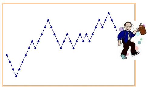
Answer: Yes, I dealt with some "random walk" of point, but that was and still is very much outside of known research (Physical Infor-mation, p. 79) and could be even more interesting than the book-researched stuff. I hope so.
1. A simple example of a random walk is along the abscissa, the x-axis, starting from O and with constant probability p ∈ (0, 1) a step is taken to the right, or with probability q = 1 - p a step is taken to the left.
In the first step, n = 1, the probability is p to arrive at the place x = 1, and q is the probability of arriving at the place x = -1. In the second step, n = 2, from x = 1 one can go to x = 2 then with probability p² (right to right), and we return to x = 0 with probability pq (right to left). In the second step, we reach x = 0 with probability qp (left to right) and the total probability that we will be back at the beginning with the second step is 2pq. By steps, we obtain the probabi-lity scheme:
... -4 -3 -2 -1 0 +1 +2 +3 +4 ... q p q² 2pg p² q³ 3q²p 3qp² p³
After n = 1, 2, 3, ... steps, a point that would have gone k = 1, 2, ..., n steps to the right has now taken n-k steps to the left. This is the Bernoulli distribution, the probability:
$$ P(k,n) = \binom{n}{k}p^kq^{n-k} $$that in n attempts we have k moves to the right. After n steps the point arrives at position x = k - (n - k) = 2k - n. Hence k = (n + x)/2. After an even number of n steps, the position x will be an even number, and when the number of steps is odd, then the abscissa is also odd.
2. The mathematical expectation (mean) of the position of a point after n ∈ ℕ random steps, of which k are to the right with probability p ∈ (0, 1), and there-fore n - k to the left with probability q = 1 - p, is μn = n(p - q). The proof of the statement is in the book Physical Information (Theorem 2.5.16). In the same book, the following theorem states that the variance of such a distribution is σn² = 4npq.
For example, when the chances of wandering left and right are equal, p = q = 1/2, then the random point (μn = 0) is expected to be at the starting point with a dispersion σn = √n. If we look at the distances of two such random walks, points that would start from different positions, this means that they will so-oner or later meet. Or, we popularly say that a drunkard will still reach home by randomly staggering. However, if moving to the right is more likely than moving to the left, p > q, then the point will move to the right as expected.
3. Mathematics describes the cosmos with absurd accuracy ... even when it ma-kes no sense to follow our equations. Nobel laureate physicist Eugene Wigner called it "the unreasonable efficiency of mathematics." If only for that reason, it would be worth mentioning the consistency of the uncertainty relations, Δp⋅Δx ≈ h, the rate of change of the mean of a random walk, μn = n(p - q), and the basis of this theory that information is the fabric of space, time, and matter, and that uncertainty is its essence, that is, that objective coincidences exist. In this relation we have in particular a higher probability (movements to the right, p - q > 0) with a smaller wavelength (λ = h/mv, v ∼ p - q), i.e. a higher certainty when the wavelength is smaller, or see the appendix to the famous Compton Effect in my book Space-Time (p. 34), or the not-so-old blog (Catch a Light).
4. But the main part of this "random walk" is not those details, but the Shann-on and physical information of that distribution, in that order:
$$ S(n) = -\sum_{k=0}^n \binom{n}{k}p^kq^{n-k}\log_b \binom{n}{k}p^kq^{n-k}, $$ $$ L(n) = -\sum_{k=0}^n \binom{n}{k}p^kq^{n-k}\log_b p^kq^{n-k}. $$This is information of the binomial distribution, the second of which is the result L(n) = nL(1). The proof is in the book Physical Information, Theorem 2.3.6. It was then and still is a new type of information called "physical" bec-ause of the additivity L(n1 + n2) = L(n1) + L(n2) from which the conservation law follows.
Random Walk II » srb
Question: Do you have anything to say about a 2-dim "random walk"?
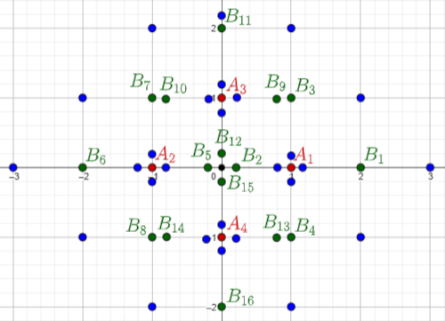
Answer: As in the case of 1-dim, free walking along the abscissa (x-axis), we consider the rectangular 2-dim system (xy-plane) discretely. As random moves, to the right and left the probability px and qx, and up and down the probability py and qy. These four numbers are positive and sum to one. In 3-dim motion, randomness would have six such numbers. In general, d-dim motion would have 2d. The graph on the left shows red points (A1, ..., A4) after one step, and green points (B1, ..., B16) after two steps. Blue are three-steppers. Their order is defined below.
All reality as we concretely perceive it, which physically interacts, is always of finite divisibility (Packages), unlike its "remainder" (an immeasurably larger part) which also contains infinities. Such finitudes are consequences of the law of conservation and we usually do not notice them, we do not have to when they are consistent with the society of large numbers.
1. We have seen that the random walk along the abscissa is in each nth step in some Bernoulli distribution ℬ(n, p). Here, p ∈ (0, 1) and 1 - p are the probabi-lities of steps to the right and to the left:
$$ (p + q)^n = \sum_{k=0}^n \binom{n}{k}p^kq^{n-k}, \quad q = 1 - p. $$The sums $P_k = \binom{n}{k}p^kq^{n-k}$ are the probability distributions of that "wobble".
Let us choose for individual moves random variables X1, X2, ..., Xn ∈ {+1, -1}, each with the same expectation μ1 = E[X1] = p⋅(+1) + q⋅(-1) = p - q. Hence aft-er n steps we have E[∑k μk] = ∑k E[μk] = n(p - q), i.e. the range n multiplied by the speed of a single step (p - q). The Variance of a variable is:
σ1² = E[(X1 - E[X1])²] = = p(+1 - (p - q))² + q(-1 - (p - q))² = p(q + q)² + q(-p - p)² = 4pq² + 4qp² = 4pq(p + q), σ1² = 4pq.
Hence the sum of n of them, the variance of a 1-dim "random walk":
σn² = E[(X - E[X])²] = nσ1², σn² = 4npq,
and these results, expectations μn = n(p - q) and variances σn² = 4npq, are equal to those in the previous answer, now derived in a different way.
2. It is similar to a "random walk" in the xy plane, then with probabilities px, qx, py, qy ∈ (0, 1) of movement right, left, up and down, px + qx + py + qy = 1. The distribution is similar to Bernoulli's:
$$ (p_x + q_x + p_y + q_y)^n = (p_x + q_x + p_y + q_y)\cdots(p_x + q_x + p_y + q_y), $$where we form the probabilities by taking one of the four sums from each of these n brackets, which become the factors. The probability of a sequence of consecutive and independent events is the product of the probabilities of those events. The list resembles counting n-digit numbers in base four. For example, for n = 1, 2, 3, ... we have 4n positions, respectively:
1 2 3 4;
11 12 13 14, 21 22 23 24, 31 32 33 34, 41 42 43 44;
111 112 113 114, 121 122 123 124, 131 132 133 134, 141 142 143 144, 211 212 213 214, 221 222 223 224, 231 232 233 234, 241 242 243 244, 311 312 313 314, 321 322 323 324, 331 332 333 334, 341 342 343 344, 411 412 413 414, 421 422 423 424, 431 432 433 434, 441 442 443 444;
Permutations of the same numbers add up to equal outcomes. So we have, 123 132 213 231 312 321, all six of which go from the starting point to the same po-int. According to the description above, these are 2-dim moves, three steps fr-om O(0, 0), in order:
123: px⋅qx⋅py right-left-up, point (0, 1), 132: px⋅py⋅qx right-up-left, point (0, 1), ... 321: py⋅qx⋅px up-left-right, point (0, 1),
and we have 3! = 1⋅2⋅3 = 6 ways to get to the same place. When only two possi-bilities are repeated, for example, 224 242 422, all three, $\binom{3}{2}$ = 3!/(1!⋅2!) = 3, lead to the same point (-2, -1) by different paths:
224: qx⋅qx⋅qy left-left-down, point (-2, -1), 242: qx⋅qy⋅qx left-down-left, point (-2, -1), 422: qy⋅qx⋅qx down-left-left, point (-2, -1).
Therefore, the summands of the nth power of a given sum of four probabilities have much fewer than they would for the n-digit base 4 listed numbers above.
3. Let us define the values of individual steps Xk ∈ {$\pm\vec{e}_x$, $\pm\vec{e}_y$}, k = 1, 2, 3, ..., using the unit vectors $\vec{e}_x$ and $\vec{e}_y$ of the coordinate axes. As in 1-dim (2), now in 2-dim random walk we find the expectation of each of the steps:
$$ \vec{\mu}_1 = E[X_1] = (+\vec{e}_x)p_x + (-\vec{e}_x)q_x + (+\vec{e}_y)p_y + (-\vec{e}_y)q_y, $$ $$ \vec{\mu}_1 = (p_x - q_x)\vec{e}_x + (p_y - q_y)\vec{e}_y. $$The expectation V = X1 + X2 + ... + Xn, the sum of n steps, is:
$$ \vec{\mu}_n = E[V] = E[X_1 + X_2 + ... + X_n] = E[X_1] + E[X_2] + ... + E[X_n], $$ $$ \vec{\mu}_n = n\vec{\mu}_1. $$As a reminder, these four probabilities are non-negative numbers with a sum of one, px, qx, py, qy ≥ 0 and px + qx + py + qy = 1, so the velocity of the "rand-om walk" is now the vector $\vec{v} = (p_x - q_x, p_y - q_y)$, and its expected range aft-er n steps is the vector $n\vec{v}$.
4. The variance of the random value Xk ∈ {$\pm\vec{e}_x$, $\pm\vec{e}_y$} at each individual step k = 1, 2, 3, ... is the same:
$$ \sigma_1^2 = E[(X_1 - E[X_1])^2] = $$ $$ = p_x\|\vec{e}_x - \vec{\mu}_1\|^2 + q_x\|-\vec{e}_y - \vec{\mu}_1\|^2 + p_y\|\vec{e}_y - \vec{\mu}_1\|^2 + q_y\|-\vec{e}_y - \vec{\mu}_1\|^2 $$ $$ = p_x[(1-p_x+q_x)^2+(p_y-q_y)^2)] + q_x[(1+p_x-q_x)^2+(p_y-q_y)^2] + $$ $$ + p_y[(p_x-q_x)^2+(1-p_y+q_y)^2] + q_y[(p_x-q_x)^2+(1+p_y-q_y)^2] $$and after editing this expression, we easily find:
$$ \sigma_1^2 = 1 - (p_x-q_x)^2 - (p_y-q_y)^2, $$ $$ \sigma_1^2 = 1 - \|\vec{\mu}_1\|^2. $$The variance of the sum of n random values Xk is σn² = nσ1².
5. For example, when the probabilities of moving left and right are equal (px = qx) and also the probabilities of stepping up and down (py = qy), even if movi-ng right is not as probable as moving up, there will be an overall expectation $\vec{\mu}_n = 0$ with variance $\sigma_n^2 = n$. Again, the mean deviation from the expected value is $\sigma_n = \sqrt{n}$. These expectations, in the 2-dim plane, are analogous to the 1-dim axis. A drunkard staggering symmetrically will sooner or later retu-rn home. Analogously, two people staggering around the park will sooner or later collide.
Another example, when there is no vertical motion then we have p'y = q'y = 0 and p'x + q'x = 1, so the 2-dim expectation lower to 1-dim, $\vec{\mu}'_n = n(p'_x - q'_x)\vec{e}_x$, and the variance:
$$ (\sigma'_n)^2 = n[1 - (p'_x - q'_x)^2] = n[(p'_x + q'_x)^2 - (p'_x - q'_x)^2] = 4np'_xq'_x. $$Symmetric movements are those that are equally likely in both directions of each of the d axes (p1 = q1, ..., pd = qd) and for an arbitrary number d = 1, 2, 3, ... of dimensions they all have expectations μn = 0 and variances σn² = n, but for d ≥ 3 the return to the starting position will not be certain.
Random Walk III » srb
Question: Why do "random walks" get lost in 3-dim?
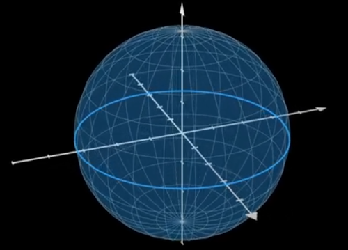
Answer: These are symmetric ran-dom movements of each of the re-ctangular coordinates, when all steps, towards each of the directi-ons of the axes, have equal proba-bilities. A point in a 1-dimensional system (along the x-axis) can go left or right, there are only two possi-bilities, each with probability 1/2. Points in a 2-dimensional system (the xy plane) have four possibili-ties and 1/4 probability. 3-dimens-ional space has six directions (left and right, there and here, up and down), each with probability 1/6. In general, in d-space a point has 2d directions, each with probability 1/2d. With larger d, the chances of a stray point finding its way back are smaller.
1. The explanations of the link in the video of this image (up right) and similar ones, take the origin O of the coordinate system as the initial positions of the points. You will notice that the point that would return has an equal number of moves in (each of) the positive and negative directions, so that the return is not possible in an odd number of steps, but in 2n of some of n = 1, 2, 3, ..., wi-th an outcome of probability (1/2d)2n, in a space with d = 1, 2, 3, ... dimensio-ns. The probability that some outcome of probability p will occur twice in a row is p², and three times in a row is p³ etc. However, we need to calculate how many ways the aforementioned sequence of 2n steps back to the starting point can be achieved, each with probability $(\frac{1}{2d})^{2n}$.
In the previous two answers about "free running" we had variables for each of the individual steps Xk ∈ {+1, -1}, where k = 1, 2, ..., 2n, with the expectation of each μ1 = E(X1) = 0 and the variance σ1² = 1. The sum of the first 2n steps is the aggregate random variable S2n = X1 + ... + X2n with the expectation:
$$ \mu_{2n} = E[S_{2n}] = E[X_1] + ... + E[X_{2n}] = 2n\mu_1 = 0. $$The variance in 2n steps is σ2n² = 2n. Namely:
$$ \sigma_{2n}^2 = E[S_{2n}^2] = E[(\sum_{k=1}^{2n} X_k)^2], $$ $$ \sigma_{2n}^2 = E[(\sum_{k=1}^{2n} X_k^2] + E[\sum_{i\ne j} X_iX_j], $$ $$ \sigma_{2n}^2 = 2n. $$In the first sum, each square is +1, and in the products on the right there are as many as +1 and -1, and their expectation is zero. The variance is σ2n² = 2n at every even 2n steps, i.e. the standard deviation is $\sigma_{2n} = \sqrt{2n}$.
2. In the case of movement along only one axis, it follows from the above that the probability of arriving at the starting point in a single case in 2n steps is P2n ≈ (2n)-1/2. For a longer walk, otherwise independent n ∈ ℕ, we find that the cumulative chance diverges:
$$ P_2 + P_4 + P_6 + ... = \frac{1}{\sqrt{2}} + \frac{1}{\sqrt{4}} + \frac{1}{\sqrt{6}} + ... \to \infty, $$that is, it reaches probability 1 (and exceeds it), which means that the point is certain to return to the starting point. One way to move to 2-dimensional spa-ces is to consider two independent perpendicular axes, each with the same probability, and these give a random point the probabilities (P2n)² = (2n)-1, now with the sum:
$$ \sum_{n=1}^\infty \frac{1}{2n} = \frac12 + \frac14 + \frac16 + ... \to \infty, $$which also diverges, i.e. reaches 1 and exceeds it, the certainty that the point will return to where it started. Let's see what happens when the three axes are random movements. The expectations and variances remain the same, but the chances of returning are smaller, (P2n)³ = (2n)-3/2, because there are more ch-oices and so many that the sum of the probabilities is insufficient to guarantee the certainty of returning:
$$ \sum_{n=1}^\infty \frac{1}{(2n)^{3/2}} = \frac{1}{2^{3/2}} + \frac{1}{4^{3/2}} + \frac{1}{6^{3/2}} + ... \lt \infty. $$The given method is still “instructive”, because the probability we use is a ro-ugh estimate, but it helps us understand what happens when the number of dimensions of the free-walk space increases. Although the mean value of all possible positions is zero, when a point starts its random walk, in a space of higher dimensions it has less and less chance of finding itself back at the st-arting point. And many other points are non-repeatable for it, simply put, there are too many of them.
3. Let's now pose the problem from the given question a little differently, first with only 1-dim random steps along the abscissa. A point that would thus ret-urn to the starting position would have an equal number of steps (say n = 1, 2, 3, ...) both to the right and to the left. As when, but it would always be a total even number of steps 2n. Each such step has a probability of 1/2, so a seque-nce of 2n such consecutive probabilities has a probability of (1/2)2n and this multiplied by the number of ways to extract n elements (steps to the right or left) from a sequence of length 2n, that is, the number of combinations, gives the probability of such a single return process:
$$ P_{2n}^{(1)} = \left(\frac{1}{2}\right)^{2n}\binom{2n}{n} = \left(\frac{1}{2}\right)^{2n} \frac{(2n)!}{n!n!}. $$So, this is the probability of a 1-dim random walk of length 2n steps. Recall that:
$$ 2^{2n} = (1 + 1)^{2n} = \sum_{k=0}^{2n} \binom{2n}{k} = \sum_{k=0}^{2n} \frac{2n\cdot(2n-1)\cdots(2n-k+1)}{1\cdot 2\cdots k}, $$and from the entire binomial sum with 2n+1 terms we now select only one, the middle and largest of the sums. Therefore each of the probabilities P2n(1) is in (0, 1), but they do not form a distribution and their sum, for all n ∈ ℕ, is not 1.
For example, two steps (2n = 2) are: right-right, right-left, left-right, and left-left. Of these four equal possibilities, two are back to the starting point. Also, $P_2^{(1)} = (2)^{-2}\binom{2}{1} = 0.5$. Of all 24 = 16 possibilities for four steps, six are back: rrll, rlrl, rdllr, lrrl, lrlr, llrr. Also, $P_4^{(1)} = (2)^{-4}\binom{4}{2} = 0.375$. Then:
$$ P_6^{(1)} = 0.3125 \quad P_8^{(1)} \approx 0.2734 \quad P_{10}^{(1)} \approx 0.2461 \ \ldots $$and the sum of the first three probabilities, $P_2^{(1)} + P_4^{(1)} + P_6^{(1)} = 1.1875$, is sufficient for the certainty of return. The sum of all diverges (Random walk 1-dim):
$$ S^{(1)} = \sum_{n=1}^\infty P_{2n}^{(1)} = \sum_{n=1}^\infty \left(\frac12\right)^{2n} \binom{2n}{n} \to \infty, $$which means that, by freely moving along one axis and infinitely stepping, the point returns to the starting point infinitely many times.
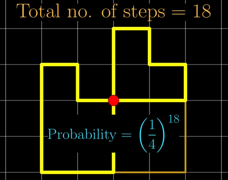
4. Let's now look at the problem of this question even more precisely. On the left, in the 2-dimensional space, there are two return paths of 10 and 8 steps, but let it be one re-turn in 18 steps and with probabi-lity 4-10⋅4-8 = 4-18. Behind the que-stion (video link), how many ways are there for such a return, in 18 random steps, and the answer is given by combinatorial calculus.
In a total of 2n = 18 steps, let there be k steps to the left and the same number to the right (here k = 4), which me-ans that there are n - k steps up and the same number down (here n - k = 5). They form a sequence of elements (right and left, up and down) that has a total of (2n)! permutations (here 18! = 1⋅2⋯18), ways of arrangement. They need to be reduced by k! due to the repetition of movements to the right and the same number to the left, and (n - k)! repetitions up and down. The prob-ability of a random sequence of 2n (here 18) steps in a 2-dimensional plane multiplied by the number of ways of formation is the probability of a single backtrack of 2n steps:
$$ P_{2n}^{(2)} = \left(\frac14\right)^{2n} \sum_{k=0}^n \frac{(2n)!}{k!k!(n-k)!(n-k)!}. $$For example, $P_{18}^{(2)} \approx 0.0344$ and for twice the number of steps $P_{36}^{(2)} \approx 0.0174$, and with three times the number $P_{54}^{(2)} \approx 0.0117$. This is a slow decay similar to a harmonic series whose sum also grows indefinitely.
5. Similarly, in 3-dimensional space, the probability of the sum of all return paths of length 2n steps would be:
$$ P_{2n}^{(3)} = \left(\frac16\right)^{2n} \sum_{j,k=0}^n \frac{(2n)!}{k!k!j!j!(n-k-j)!(n-k-j)!}, $$where k is the number of steps to the right and the same number to the left, j is the number of steps there and the same number to the left, and the remain-ing n-k-j is the number of steps up and the same number to down.
The sums of the return probabilities in 2-dim and 3-dim steps are:
$$ S^{(2)} = \sum_{n=1}^\infty P_{2n}^{(2)}, \quad S^{(3)} = \sum_{n=1}^\infty P_{2n}^{(3)}. $$With the grow in the number of steps, 2n, the first sum increases sufficiently to give a good chance of the random point returning to its starting position (2-dim random walk), unlike the second. Nearly the same as in the previous exa-mple (2), it happens that returning to the starting position in a 2-dimensional random motion becomes almost certain, while in a 3-dimensional one it is not.
Fictions II » srb
Question: How do you interpret "random walks" using the definition of reali-ty?

Answer: Reality is observable, per-manent and true, but there are also other natural phenomena, and so-me of them are fictions of which we are aware through vitality. Let's try to notice them using the moment when a stone falls into water, push-ing itself into it, which creates tho-se disturbances on its surface, whi-ch we see in the picture on the rig-ht.
1. A series of such moments shapes our reality. Due to uniqueness (Informati-on Coupling, p. 124) all these realities are at least slightly different for differe-nt subjects, and even for the "same" they are not the same at different momen-ts. This constant change is a reality in which there is room for unrealities, incl-uding fictions, that is, what we perceive because we are vital. Unlike dead phy-sical nature, which has only truth, permanence and measurability, we can ad-ditionally lie, die and perceive something of the physically immeasurable.
There is also the principle of diversity, which also applies to 4-dimensional space-time. Simply put, there is no staticity in the real space-time model, at least not in the way we imagine it algebraically or geometrically when we st-ring three spatial dimensions in time according to the space-time model. Th-ere is already an interpretation of "reality" in the interpretation of the "rand-om walk". Namely, we add linear spaces in algebra by increasing their dimen-sions without making any significant changes. However, a random walk along one and within two and three dimensions is significantly different. For examp-le, in 3-dimensional space it is irreversible, while in 2-dim and 1-dim it is not.
2. There is no static 4-dimension space-time. Recent studies in quantum phy-sics suggest that on extremely small, microscopic scales, time can theoretically move in both directions, forward and backward, raising the question of a stri-ctly unidirectional "arrow of time". At these small scales, within the framew-ork of this information theory, changes were also expected during other dim-ensions of time. Different subjects see some of the same phenomena during different processes in very small portions, and we vitals, with all this and with the gift of seeing them through our fictions, also see some unrealities.
I do not overestimate these findings of "reversible time," just as I am not conc-erned with experimental confirmation of my theory; this is only consistent wi-th the hypothesis that information is the weaving of space, time, and matter, and that uncertainty is its essence. Therefore, even 4-dimensional space-time, as we imagine it today in mathematics, is not a complete description of reality. Again, even if they are just fictions, non-contradictory models can be valid.
3. Let us consider again the concentric circles around the thrown stone, and imagine them as waves on water that are spreading, with constant wavelengt-hs λ and decreasing amplitudes a. Let σ be the diameter of such a circle at a given moment, so that its circumference is 2σ, and its area σ²π/4, and then imagine them as points. In another coordinate system, they are points on the x-axis, the abscissa along which they move randomly.
If it can do that, then the positions of the "random point" pile up into the sha-pes of a Gaussian bell curve:
$$ \phi(x) = \frac{1}{2\pi}\exp(-\frac{x^2}{2}). $$The term "bell curve" is commonly used in the social sciences. It is called the normal distribution in probability theory and statistics, and in physics it is us-ually called the Gaussian distribution, although they all refer to exactly the sa-me probability distribution of independent random events with strictly given characteristics, including the fact that it is shaped like a bell. It occurs, in this case, when we consider the points on the x-axis as surfaces that cover concen-tric circles around a stone thrown into water. The free movement of such "po-ints" seems to be non-free from randomness, say, circles of "synchronized" surfaces with a normal distribution, but not the circumference.
4. In a similar situation, the expansion of concentric balls in 3-dimensional space, the mentioned region of the "random walk" is the surface of the ball. Its sphere will have an area of S = 4πr² when its radius is r, or it will have an area of πσ² if its diameter is σ. Then we see in action how "random walks" get lost in 3-dimensional space (Random Walk III). The mean value of the points of the sphere is also the center of the ball, but its surface goes away and does not return.
At the same time, we note the demonstration of the additivity of the physical information of the random walk (Random Walk, 4). In further steps r the area S of the sphere becomes larger while the exponent exp(-S) of the distribution becomes smaller. The first behaves like the number of steps n, the second is like the physical information L(n), and the third is like the exponent of the Hartley information exp(-L).
Hypergeometric » srb
Question: What about the hypergeometric probability distribution?
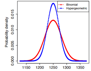
Answer: You can read about it in detail in the book Mathematics of Lottery (pp. 93-99), but I wrote it in 2013, avoiding mentioning info-rmation theory. It is a slightly more complex form of binomials, which I only discussed later in the same bo-ok (pp. 100-103), simply as less im-portant for lotto games.
In the binomial distribution, in n ∈ ℕ repetitions with replacement, fa-vorable outcomes with probability p ∈ (0, 1) are obtained and, at the same time, they are not obtained with cons-tant probability q = 1 - p. Otherwise, it is possible to have r = 1, 2, ..., n favora-ble outcomes out of n:
$$ \binom{n}{r} = \frac{n!}{r!(n-r)!} = \frac{1\cdot 2\cdots (n-r+1)}{1\cdot 2\cdots r} $$ways. This number, with the binomial “en chose ar”, is also written $C^n_r$, or nCr, and is also called the number of combinations. However, in the hypergeometr-ic distribution, the drawn event is not returned and the number of initial opti-ons n is eventually reduced to n - r.
1. In the most general case, the organizer of the lotto game n out of N random-ly draws n numbers from the set S = {1, 2, …, N}, and the player guesses m nu-mbers on his paid series of M numbers. The probability of such a random eve-nt is:
$$ \Pr[X = m] = \frac{\binom{M}{m}\binom{N-M}{n-m}}{\binom{N}{n}}, $$where X denotes the random variables of the given distribution in general, and m is the number of preferred choices among them. From the very definition of this probability it is clear that we are talking about independent possibilities and that the sum of all is one. Therefore, we have a probability distribution.
2. A more rigorous proof that this is indeed a distribution is in the mentioned Mathematics of Lottery. It is a proof of the Vandermonde's identity:
$$ \sum_{m=0}^n \binom{M}{m}\binom{N-M}{n-m} = \binom{N}{n}, $$from which it immediately follows that the sum of the above probabilities is one. In addition, there is also a proof that the mathematical expectation and variance of this hypergeometric distribution are:
$$ \mu(m) = n\cdot\frac{M}{N}, \quad \sigma^2 = n\cdot\frac{M}{N}\cdot\frac{N-M}{N}\cdot\frac{N-n}{N-1}. $$For example, Lotto Serbia (n = 7 of N = 39) uses a drum with 39 balls, and to win the jackpot you need to match 7 numbers.
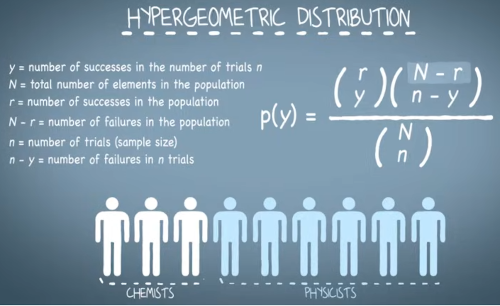
3. Perhaps an easier example is the image and link to the right. We sel-ect participants from a group of th-ree chemists (M = 3) and six physi-cists (N - M = 6), where the number of chemists is denoted by r, the nu-mber y of their successful choices (instead of m in the previous exam-ple). Above in the probability fracti-on is the numerator and the numb-er of ways to select a group of n wi-th y successes. The numerator is the number of ways to take any of these n fr-om all N. When we choose five members, two of whom are chemists, this gives N = 9, n = 5, r = 3, y = 2, N - r = 6 and n - y = 3, hence the probability:
$$ p(y) = \frac{\binom{r}{y}\binom{N-r}{n-y}}{\binom{N}{n}} = \frac{\binom{3}{2}\binom{6}{3}}{\binom{9}{5}} \approx 0,4762. $$4. The Python (3.11.0) program would be:
import math
N, n, r, y = 9, 5, 3, 2
c1 = math.comb(r, y)
c2 = math.comb(N-r, n-y)
c3 = math.comb(N, n)
print(c1*c2/c3)
# Output: 0.47619047619047616
The same program works with any other hypergeometric probability distribu-tion numbers.
5. Finally, let's briefly look at the main part of this story. Unlike the non-addi-tive Shannon information S(N) = -∑N p(N) ln p(N) of the hypergeometric di-stribution, its physical information L(N), whatever it is, must be like that. For it (in my sense) to be "physical" it is enough for it to be additive:
L(N1 + N2) = L(N1) + L(N2).
I leave open the question that there may be more of these besides the ones listed above. This means, for example, that the Serbian Lotto (2) from a drum with N = 39 balls, with all other parameters unchanged, would have to have the same physical information as two lotto drums with N1 = 20 and N2 = 19 balls, but also with some other capacities when N1 + N2 = N.
Fisher » srb
Question: How come you leave the question of physical information open without stating it?
Answer: Statements about functio-ns without their exact definition are known to mathematicians as existe-nce theorems. Non-constructive pr-oofs of existence are, for example, that a function must exist (often using an assumption as the Axiom of Choice), without providing a de-tailed algorithm, formula, or set of ordered pairs that define the functi-on specifically. I have already desc-ribed one type of alleged physical information in the book Physical Information (2.5.1 Indicators). There it was also applied to the binomial dis-tribution, on which I will now demonstrate another such one.
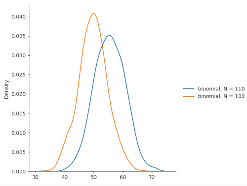
1. In the figure on the left are two distributions ℬ1(N1, p1) and ℬ2(N2, p2). Bo-th are binomial and have the same probability of successful outcomes, p1 = p1 = 1/2, but they have different total number of trials, the higher red N1 = 100 and the right-shifted blue N2 = 110. In both cases they are power expansions in sums (p = q = 0.5):
$$ 1 = (p + q)^N = \sum_{n=0}^N \binom{N}{n}p^nq^{N-n} = \sum_{n=0}^N \binom{N}{n}\left(\frac12\right)^N = $$ $$ = [\binom{N}{0} + \binom{N}{1} + ... + \binom{N}{n} + ... + \binom{N}{N}]\left(\frac12\right)^N $$ $$ = [(1 + 1)^N] \left(\frac12\right)^N = 1. $$It is intentionally written so that it can be seen that this binomial (p = 1/2, q = 1 - p) is a well-defined probability distribution $P_n = \binom{N}{n}(1/2)^N$, N = const. But also to see the importance of the binomial coefficient over (0.5)N = const.
2. In cases of very large numbers of repeated trials (N → ∞) the numbers of several changes will be negligible (ΔN/N → 0) and then we will move on to differentials (ΔN ≈ dN). Let us show that then:
$$ \frac{d}{dN}\ln\binom{N}{n} = H_N - H_{N-n}, \quad H_m = \sum_{k=1}^m \frac{1}{k}. $$These Hm are the so-called harmonic numbers. The proof is simple:
$$ \binom{N}{n} = \frac{N(N-1)\cdots(N-n+1)}{n!}, $$ $$ \ln\binom{N}{n} = \ln N + \ln(N-1) + \dots + \ln(N-n+1) - \ln n!, $$ $$ \frac{d}{dN} \ln\binom{N}{n} = \frac{1}{N} + \frac{1}{N-1} + \dots + \frac{1}{N-n+1}, $$and that is the equality sought.
3. Applied to the hypergeometric distribution, where we have four possible pa-rameters (N, M, n, m) for the probability:
$$ \Pr[X = m] = \frac{\binom{M}{m}\binom{N-M}{n-m}}{\binom{N}{n}}, $$we get different harmonic sequences. Here, n out of N possibilities are rando-mly drawn. In doing so, m successes are achieved from a set of M ≤ N desired ones. The Hartley information of this probability, -ln Pr[X = m], its logarithm, and the derivative with respect to one of the four parameters has the meaning of the rate of change of the probability depending on that parameter.
4. Like the conditional probability Pr(A|B), that a random event A occurs wh-en B occurs, i.e. the probability A under the conditions of the occurrence of a random event B, let us now observe changes in a function f(X; θ) in general by estimating the influence of the parameter θ on the variables X. When instead of changes in the function f itself we observe changes in its logarithm (ln f), because they follow each other (they grow and fall together, although at diff-erent speeds), we can observe the derivative ∂θ ln f(X; θ). When such a deriv-ative is positive, increasing θ increases f, and when the derivative is negative, increasing θ decreases f. We then find the mathematical expectation of the square of such a derivative, which is the so-called Fisher information.
$$ F(x,\theta) = E_x\left[\left(\frac{\partial}{\partial \theta}\ln f(x;\theta)\right)^2\right] = E_x\left[\left(\frac{1}{f}\frac{\partial f}{\partial \theta}\right)^2\right]. $$In the case of probability density, the expectation is the integral, and the vari-ance is:
$$ F(x,\theta) = \int(f'_\theta)^2f\, dx = \sigma_\theta^2[f'_\theta(x,\theta)], $$ $$ F(x,\theta) = -\int\left[\frac{\partial^2}{\partial x^2}\ln f(x,\theta)\right]f(x,\theta)\, dx. $$Therefore, Fisher's information F(x, θ) is such that it measures the fluctuatio-ns of the function f(x, θ) depending on the parameter θ, and is also the varian-ce (with respect to x) of the derivative of the given function with respect to θ. It is also the negative expectation of the second derivative (taken with respect to the parameter θ) of the logarithm of the given function, and it is also the expectation of the square of the first derivative.
5. Example. Let's check whether 1/σ² is the Fisher information of the normal distribution 𝒩(μ, σ²), i.e. the function:
$$ \phi(x, \mu) = \frac{1}{\sqrt{2\pi \sigma^2}}e^{-\frac{(x-\mu)^2}{2\sigma^2}}. $$Solution: Hartley information is the logarithm of the probability:
$$ I(x, \mu) = \ln \phi(x, \mu) = -\frac12\ln(2\pi\sigma^2) - \frac{(x-\mu)^2}{2\sigma^2}, $$ $$ \frac{\partial}{\partial \mu}I(x, \mu) = \frac{x-\mu}{\sigma^2} = I'(x,\mu), $$ $$ \frac{\partial}{\partial \mu}I'(x,\mu) = -\frac{1}{\sigma^2} = I''(x,\mu), $$and the expectation of this constant (the integral of the normal distribution is one) is the Fisher information:
$$ F(x,\mu) = -E[I''(x,\mu)] = \frac{1}{\sigma^2}. $$That was supposed to be shown. ∎
6. Example. Let us consider how it is otherwise shown that n/(p - p²) is the Fisher information of the binomial distribution ℬ(n, p), or the probability information:
$$ f(n,p,x) = \binom{n}{x}p^x(1-p)^{n-x}. $$Instruction: Here p is the parameter, so for the probability distribution is:
$$ \ln f(n,p,x) = \ln\binom{n}{x} + x\ln p + (n-x)\ln(1-p), $$ $$ \frac{\partial}{\partial p} \ln f(n,p,x) = \frac{x}{p} - \frac{n-x}{1-p}, $$ $$ \frac{\partial^2}{\partial p^2} \ln f(n,p,x) = -\frac{x}{p^2} - \frac{n-x}{(1-p)^2}, $$so we next take one trial, n = 1, to find the expectation:
$$ F(1,p,x) = -E\left[-\frac{x}{p^2} - \frac{1-x}{(1-p)^2}\right] = \frac{p}{p^2} + \frac{1-p}{(1-p)^2}, $$ $$ F(1,p,x) = \frac{1}{p(1-p)}. $$Hence, we simply take F(n, p, x) = n/(p - p²), for n repetitions of a unit expe-riment. For a more rigorous explanation, the so-called informant is used, and the corresponding so-called score statistics. This, Fisher's information of the binomial distribution, is also some physical information and we note that it has a different form than mine, mentioned earlier.
Influence II » srb
Question: Fisher's information measures the mutual influence of variables?
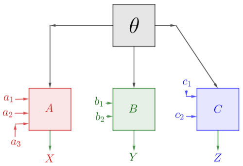
Answer: Yes, you could say that. Fisher information:
$$ F(X |\theta) = E_x[(\partial_\theta \ln f(X | \theta))^2] $$or the expectation of the square of the change in the function f(X|θ), due to changing X (one or more variables), when changing the pa-rameters θ (one or more of them).
The figure on the right shows a sketch of the influence of the parameter θ, e.g. the average intelligence of the population, on the economic development of the country A, where a1 is the influence of institutions, a2 geography, a3 history, and so on. Then, on the birth rate B, where b1 is the size and age of the population, b2 is access to ed-ucation and career opportunities for women, or the like. Then C, on mortality from cancer and heart attacks, where c1 is unhealthy diet, c2 is air pollution, and so on. We express these phenomena (A, B, C) by the quantities X, Y, or Z and look for the influence of the parameter θ on them. Analogous, for examp-le, is the influence of vitality on global phenomena (Influence). This is what the use of Fisher information is about.
1. The normal distribution (bell-shaped, Gaussian curve) is widely used to model natural and social phenomena where data are clustered around a ce-ntral mean value, such as human height, IQ scores, and measurement errors. It is essential for quality control in manufacturing and calculating insurance risk, or determining percentiles of test scores and analyzing scientific data.
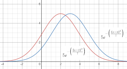
In the image on the left are two Gaussian normal distribution curves:
$$ \phi(x; \mu, \sigma) = \frac{1}{\sqrt{2\pi}\sigma}e^{-\frac{(x-\mu)^2}{2\sigma^2}}. $$On the left is red with expectation μ1 = 2 and on the right is blue with expectation μ2 = 3, and both have variances σ² = 3.5. When μ is the Fisher information parameter, we calculate:
$$ F(x | \mu) = E_x[(\partial_\mu \ln \phi(x;\mu,\sigma))^2] = $$ $$ = E_x\left[\left(-\frac{\partial}{\partial \mu} \frac{(x-\mu)^2}{2\sigma^2}\right)^2\right] = E_x\left[\left(\frac{x-\mu}{\sigma^2}\right)^2\right] $$ $$ = \frac{1}{\sigma^4}\int_{-\infty}^{+\infty} (x-\mu)^2\phi(x;\mu,\sigma)\, dx , $$and this integral is the variance, that is σ², so finally:
$$ F(x|\mu) = \frac{1}{\sigma^2}. $$Therefore, the Fisher information decreases with the square of the standard deviation σ of the Gaussian curve, i.e. with its variance. If the Gaussian curve is lower, with a flatter bell curve, then its variance is higher and the gap betw-een the two curves in the image would appear smaller. The more horizontal the graph, the smaller the shift in the mean value μ would be, its Fisher infor-mation is reduced, and the influence of the parameter μ on the shape of the graph is smaller.
2. We will call the functions ℓx(θ) = ln ℒx(θ), the random variables, “log likeli-hood”, and the functions s(θ) = ∂θ(θ), which are their derivatives, “score”. The maximum log-likelihood (MLE) value is obtained by equating the score to zero and solving for θ, whereas Fisher's information is the variance of the score fu-nction. It is known that when the derivative of an integral is the integral of the derivative, ∂θ ∫ fθ(x) dx = ∫ ∂θ fθ(x) dx.
Hence, for the probability density functions (pdf) we have:
$$ \int f_\theta(x)\, dx = 1 \quad \to \quad \int\frac{\partial^k}{\partial \theta^k} f_\theta(x)\,dx = 0, $$for consecutive derivatives (k = 1, 2, 3, ...), i.e. $\int f'\,dx = 0$, $\int f''\,dx = 0$, ..., so for ℓ = ln f we find the derivatives and expectations:
$$ \ell' = \frac{f'}{f}, \quad \ell'' = \frac{f''}{f} - \left(\frac{f'}{f}\right)^2, $$ $$ E[\ell'] = \int \ell' f\, dx = \int \frac{f'}{f}\cdot f\,dx = \int f'\,dx = 0, $$ $$ E[\ell''] = \int f''\,dx - E[\left(\frac{f'}{f}\right)^2] = -E[\left(\frac{f'}{f}\right)^2] = -E[\ell'^2] = -\text{Var}[\ell']. $$So, the expectation of the second derivative is the variance of the scores, or rather the first derivative of the logarithmic likelihood function, exactly what we had for Fisher information (Fisher, 4), now slightly differently. I mention this to be an aid for possible calculations when applying it, in estimating the mutual influences of variables.
3. The law of large numbers of probability theory states that the quotient of a given and all outcomes of a random event groups around the probability of the given event when the random experiment is repeated. In the "informatics con-cept", prioritizing time (repeated news is stale), it is the effect of past events on present events and the emergence of reality, or the transfer of information that speaks of their mutual influence. Here we are at Fisher's information and the answer to the question posed.
Consider a random function of some parameter θ defined by n-tuples (sets) of variables X1, X2, ..., Xn, but which is the product of the individual ones:
$$ f_\theta(x_1, x_2, ..., x_n) = \prod_{k=1}^n f_{\theta,k}(x_k), $$ $$ \ell_{n,x}(\theta) = \ln f_\theta(x_1, x_2, ..., x_n) = \sum_{k=1}^n \ln f_{\theta,k}(x_k), $$ $$ \ell'_{n,x}(\theta) = \sum_{k=1}^n \frac{\partial}{\partial \theta} \ln f_{\theta,k}(x_k), \quad \ell''_{n,x}(\theta) = \sum_{k=1}^n \frac{\partial^2}{\partial \theta^2} \ln f_{\theta,k}(x_k). $$The law of large numbers says that the sample average over a long period of repeated experiments becomes the theoretical average, the expected value. The first derivation, that equality on the left, is about the mean. Here's why the Fisher information of the binomial distribution (Fisher, 6) holds:
F(n, p, x) = nF(1, p, x) = n/(p - p²),
because in general it holds that F(n|θ) = nF(1|θ). The sample size n times re-peated becomes n times repeated unit sample. We understand this statistica-lly.
For example, as of 2022-2023, the average life expectancy taken at the global level is approximately 72–73 years, but the average life expectancy in Serbia was 75-76 years. The mean value in the wider population does not necessarily match the estimate in a smaller sample, but by taking a larger and larger sam-ple, an increasingly better match occurs.
In this regard, let's look at these laws, for example, that the Fisher information of the normal distribution (1), with repetition which in a single experiment is F(x|μ) = 1/σ², by repetition will lose influence of the dispersion (as σ → 0) and grow. Or, when repeating a measurement, in which we certainly make measu-rement errors, in order to take the average value of the measurements and get a more accurate result and be better informed about the real value. I repeat, it is also about the influence of the past on the present.
4. Finally, there is the central limit theorem (CLT), which states that the distri-bution of sample means approaches a normal distribution (bell curve) as the sample size becomes larger (n ≥ 30), regardless of the underlying population distribution. As the sample size increases, the mean of the sample means app-roaches the population mean (μ), while the standard deviation (the dispersion σ) decreases. All samples are independent and drawn at random, so the stand-ard error, the variance of the sample mean, becomes σx̄ = σ/√n. Hence:
$$ F_n(x|\mu) = nF_1(x|\mu) = \frac{n}{\sigma^2}, $$in general, in the Fisher information many, n times, repeated distributions for which the central limit theorem holds. In particular, it is the equality:
$$ F(n,p,x) = nF(1,p,x) = \frac{n}{p(1-p)} $$in the aforementioned (3) Fisher information of the binomial distribution. Th-is section is a contribution to the previous answer (Fisher) to the question of "physical" information that was not previously explicitly stated.
Accumulation » srb
Question: Isn't it paradoxical that by reducing uncertainty by repeating an experiment, the "information" increases, which is supposedly the "amount of uncertainty"?
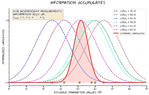
Answer: The image link on the rig-ht may help you answer the questi-on. The Fisher information F(X|θ) is which represents the amount of action of some parameter θ on the variable x ∈ X of the given function f(x|θ). The image of multiple dotted bells, the density of repeated trials, produces a red solid and steeper li-ne above the shaded area of the be-ll-shaped distribution that comes from the central limit theorem (CLT). The Fisher information is simply a mea-sure of these actions, the accumulation of dotted graphs on the solid.
1. We know that the Shannon (average Hartley) information of meaningful te-xt is less than the same volume of random text (Voltage). This reveals to us a way of recognizing vitality among dead physical substance, because this is a property of meaningful actions in general. The loss of information can be achi-eved from its previous excess, just as a sharp object can penetrate deeper from a run, and this power comes from the excess amount of choice that living bei-ngs have in relation to inanimate ones. After all, the ability to fantasize, lie and be dishonest (Honesty) comes with this excess of information that living bein-gs have in relation to the inanimate physical substance of which they are also composed. We see this in that pointed bell in the picture above, the accumula-ted influence of previous duller bells; greater focus extracted from greater di-spersions.
2. When it exists, the derivative of a function is the slope of the graph, the tan-gent of the angle between the tangent line to the graph and the abscissa, at a given point. It is the score s(θ) = ∂θ ℓx(θ) the random function ℓx(θ) = ln ℒx(θ) which is the logarithm of the probability function ℒx(θ). We can see this in the previous answer (Influence II, 2), as well as the proof that the expectation of the score must be zero, E[ℓ'] = 0. Intuitively, this tangent is horizontal (parallel to the θ-axis) at the mean, at the top of the bell, and positive for the increasing graph before and negative for the decreasing graph after. It is symmetrically positive-negative for the cumulative expectation to be zero, which implies av-eraging over repeated trials.
Namely, individual distributions that would have slower graph rises before the maximum would have smaller parameter influences there and a smaller sink of the final action on the Fisher information, and vice versa. The compensati-on of these influences leads to the symmetry of negative and positive slopes, and to zero expectation. This “accumulation symmetry” has its another story.
3. A function is a mapping of one or more originals into at most one copy. Th-us f1(x) = x² a function that copies both numbers +3 and -3 into the number +9, and the function f2(x, y) = log2(xy) maps x = 2 and y = 4, or x = 4 and y = 2, and many other pairs into the same number 3. Let f3(x, y, z) be a function whose three variables are x(t), y(t) and z(t) in the manner of a function depe-ndent on the parameter t. This means that by the chain rule of this function with respect to the parameter is:
$$ \frac{df_3}{dt} = \frac{df_3}{dx}\frac{dx}{dt} + \frac{df_3}{dy}\frac{dy}{dt} + \frac{df_3}{dz}\frac{dz}{dt} = \vec{f'}\cdot \nabla. $$It is the scalar product of the vectors, the derivative of a function, and the operator:
$$ \vec{f'} = (f'_x, f'_y, f'_z), \quad \nabla = (d_t, d_t, d_t). $$Applying the function ℓ(t) = ln f(t) and E[ℓ'] = 0 to the score gives that the exp-ectation of the log-likelihood (log-likelihood), and then the probability itself of a given distribution, is the "surface" (the number of variables is not always th-ree) to which the gradient of the parameter's action quantity (Fisher informa-tion) would be perpendicular. The scalar product is zero only of perpendicular vectors.
4. When functional, the influence of the parameter (θ) on the logarithm of the probability ℓx(θ) = ln ℒx(θ), i.e. on the score function s(θ) = ∂θ ℓx(θ), behaves like a force field. This is quite acceptable in this information theory, where in-formation is observed in packets of actions, quanta ΔE⋅Δt = h and in general some products of changed energy (ΔE) for the elapsed time (Δt). This mutual action, the parameter on the probability function, is calculated by Fisher info-rmation. It does not express information in a general sense (if such a thing existed), but as a mutual influence.
Poisson » srb
Question: Explain the Poisson distribution to me?
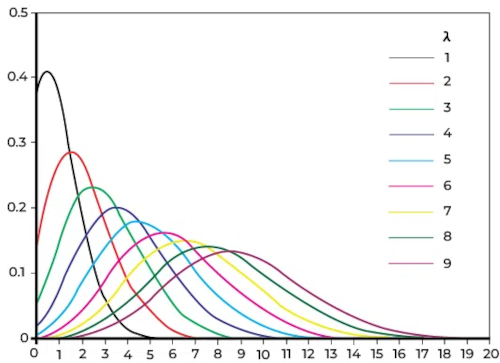
Answer: In the extreme case, let's say n > 50 and a small expectation µ = np < 10, the binomial distribu-tion becomes Poisson, but other-wise (µ ≥ 10) it becomes normal, the so-called Gaussian (Quantum Mechanics, p. 75). There is n the number of trials, with p ∈ (0, 1) the probability of the desired outcome, and q = 1 - p the probability of the unfavorable one. The expectation μ = np and the variance σ² = npq for the binomial are equal to μ = σ² = λ for the Poisson distribution.
The figure on the left shows the graph of the Poisson distribution:
$$ P(X=k) = \frac{\lambda^ke^{-\lambda}}{k!}, \quad k = 1,2,3,...,n \to \infty, $$in turn for all λ = 1, 2, ..., 9. With increasing expectation λ = E[P] = np, the vertex of the graph shifts to the right and its maximum decreases, but the area under (always unitary) expands above the abscissa, because its variance σ² = λ increases.
1. Let's find the Fisher information F(X|λ) of the Poisson distribution given the set of trials X = (X1, ..., Xn). We know that F(X|λ) = nF(X1|λ), so let's find first the information of just one sample F(X1|λ):
$$ f(x|\lambda) = \frac{\lambda^xe^{-\lambda}}{x!}, $$ $$ \ln f(x|\lambda) = x\ln \lambda - \lambda - \ln x!, $$ $$ \frac{\partial}{\partial \lambda}\ln f(x|\lambda) = \frac{x}{\lambda} - 1, $$ $$ -\frac{\partial^2}{\partial \lambda^2}\ln f(x|\lambda) = \frac{x}{\lambda^2}. $$Hence the Fisher information of a sample of the Poisson distribution:
$$ F(X_1|\lambda) = -E_\lambda\left(-\frac{\partial^2}{\partial \lambda^2}\ln f(X_1|\lambda)\right) = E_\lambda\left(\frac{X_1}{\lambda^2}\right) = \frac{\lambda}{\lambda^2}, $$ $$ F(X_1|\lambda) = \frac{1}{\lambda}. $$So, the Fisher information of an n-tuple of the Poisson distribution is:
$$ F(X|\lambda) = nF(X_1|\lambda) = \frac{n}{\lambda}. $$It is information from a series of experiments X = (X1, ..., Xn).
2. Poisson distributions are often used for counting data. These are statistics with the numbers k = 0, 1, 2, 3, ..., such as Ladislaus Bortkiewicz who, in the late 19th century, investigated the accidental deaths of Prussian soldiers due to horse kicks. He analyzed 20 years of data in 10 army corps, equivalent to 200 years of observation of one corps. He found that on average 0.61 soldiers per corps died from horse kicks each year, but most years no soldiers died. On the other hand, in one tragic year, four soldiers in the same corps died from horse kicks. He (Bortkeiwicz) was the first to use this distribution.
3. For example, web hosting companies use the Poisson distribution to model the number of expected visitors per hour that web pages will receive. If a given website has an average of 20 visitors per hour, we can use the Poisson distrib-ution Calculator to find the probability that it has more than a certain number of visitors in a given time:
- P(X > 25 visitors) = 0.11218
- P(X > 30 visitors) = 0.01347
- P(X > visitors) = 0.00080
This gives hosting companies an idea of how much bandwidth they need to provide to different websites to ensure specific numbers of visitors each hour.
4. The Poisson process meets the following criteria:
- Events are independent of each other. The occurrence of one event does not affect the probability of the other event occurring.
- The average rate (events per time period) is constant.
- Two events cannot happen simultaneously.
Here are some examples from exercises by students at FIU.
4a. Example. On an average workday, a waitress does not receive tips from 5 customers. Calculate the probability that she does not receive tips from 7 cust-omers today.
Solution: The waitress has an average of 5 customers per day who do not tip: λ = 5. The random variable X = 7 is the number of customers who would be there today without leaving a tip, and we are interested in:
$$ P(X = 7) = \frac{e^{-\lambda}\lambda^k}{k!} = \frac{e^{-5}\cdot5^7}{7!} \approx 0.10444. $$With that probability, there are not exactly 7 tips in one of the ten days. ∎
4b. Example. During a typical football game, a coach expects about 3.2 inju-ries. Let's calculate the probability that the team will have at most 1 injury in this game.
Solution: Now λ = 3.2. We are interested in the probability:
$$ P(X \le 1) = \sum_{k=0}^1\frac{e^{-\lambda}\lambda^k}{k!} = \frac{e^{-3.2}\cdot 3.2^0}{0!} + \frac{e^{-3.2}\cdot 3.2^1}{1!} \approx 0.17120. $$With that probability, at most one player injury occurs in about one in 5.8 games. ∎
4c. Example. A small life insurance company has an average of six death cla-ims per day. Find the probability that it will receive at least seven deaths on a randomly selected day.
Solution: This is the probability that there will be no more than six or fewer:
$$ P(X ≥ 7) = 1 - P(x ≤ 6) \approx 0.39370, $$which happens once every 2.54 days on average. ∎
|
|
|