|
|
|


Clarity » srb
Question: What is good for signal clarity?

Answer: Technically speaking, if you choose higher-speed transmi-tters with less technical interfere-nce and send codes of shorter len-gths, the recommendations will be of greater range, therefore improvi-ng the quality of data transmission.
1. I will demonstrate this on a binary symmetric channel matrix:
\[ K(t) = \begin{pmatrix} \frac{1 + e^{-2\lambda t}}{2} & \frac{1 - e^{-2\lambda t}}{2} \\ \frac{1 - e^{-2\lambda t}}{2} & \frac{1 + e^{-2\lambda t}}{2} \end{pmatrix}. \]This is an example of a double stochastic matrix, a complete Markov chain. Its columns (these and rows) represent probability distributions; they are positive numbers summing to one. Multiplying by it vectors that are probability distri-butions, we also get distributions. Independent of the input probabilities, say p = (p1, p2), for t → ∞, we get the output distribution q* = (1/2, 1/2). It then becomes a "black box," a transmitter whose output tells us nothing about the input.
If the time t > 0 transmission is shorter; also, if the transmission interference λ > 0 is less, and the fewer transmission elements, the closer the copy is to the original. It follows from:
\[ \begin{pmatrix} \frac{1 - e^{-2\lambda t}}{2} + e^{-2\lambda t}p \\ \frac{1 + e^{-2\lambda t}}{2} - e^{-2\lambda t}p \end{pmatrix} = \begin{pmatrix} \frac{1 + e^{-2\lambda t}}{2} & \frac{1 - e^{-2\lambda t}}{2} \\ \frac{1 - e^{-2\lambda t}}{2} & \frac{1 + e^{-2\lambda t}}{2} \end{pmatrix} \begin{pmatrix} p \\ 1 - p \end{pmatrix}, \]as well as from the fact that every part of the message is transmitted in this way and that then the probability of correct transmission is the product of particular probabilities.
2. Theorem. (Exponential process) When the probability of occurrence of a signal is F(t), a continuous and increasing function of time is such that:
(i) independent of the beginning of the period t, (ii) independent of previous signals,
then F(t) = 1 - eλt, where λ is a non-negative real number.
Proof: Let us denote by p the probability that the signal will not appear in a period of unit length t = 1, and divide the period itself into n of equal disjoint intervals. Let us denote by p0(1/n) the probability that the signal will not app-ear in the period t = 1/n. Due to the independence conditions, (i) and (ii), is:
\[ p = \left(p_0(\frac{1}{n})\right)^n, \quad p_0(\frac{1}{n}) = p^{\frac{1}{n}}. \]Hence, for any k = 1, 2, 3, ..., the probability that the signal will not appear for time t = k/ n equals:
\[ p_0(\frac{k}{n}) = p^{\frac{k}{n}}, \quad F(\frac{k}{n}) = 1 - p^{\frac{k}{n}}, \quad \lambda t = -\frac{k}{n}\ln p, \]and that is what had to be proved. ∎
3. The continuous binary symmetric channel matrix (1) is a typical Markov chain, as seen from theorem (2), for memoryless channels. When the lambda parameters in the columns are different, we do not have symmetry. In a multi-line situation there is no binary; we have multiple disjoint outcomes. Each of these possibilities maintains the above conclusion, that (a) data transfer is more accurate with a higher speed transmitter, with (b) less technical interference (lambda), and with (c) a smaller code length (n ∈ ℕ).
Due to the Borel–Cantelli lemma, that only finitely many events of infinite distribution can be realized with probability 1, the third (c) of the above conditions is not as important as it seems at first glance. Cases with large n code lengths will have fewer signals transmitted with a probability greater than zero. However, situations n → ∞ they are more realistic, although we often do not notice these many ways of perception around us.
Fading » srb
Question: Can you elaborate a bit on the channels of the above type?
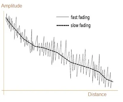
Answer: The temporal variation of received signal strength due to cha-nges in transmission media, or pat-hs, is called fading. Fading depends on various factors. In the fixed sce-nario, degradation (of wireless tra-nsmission) also depends on weath-er conditions such as precipitation, lightning, etc. Wireless fading sce-narios depend on obstacles in the way, or wired on the structure of the message carrier.
1. What we are particularly intere-sted in are channels, K = (κij), of the above type:
qj(t) = ∑i pi κij(t),
indices i, j = 1, 2, ..., n, are the distribution ranges p = (p1, p2, ..., pn), or the value of the parameter t when the output signal is no more similar to the starting:
\[ \frac{dq_j(t)}{dt} = \sum_i p_i\cdot\frac{d\kappa_{ij}(t)}{dt} = \sum_i p_i \cdot \sum_l \kappa_{il}(t) = \sum_{i,l} p_i \cdot \kappa_{il} \cdot\lambda_{lj}, \] \[ \frac{dq_j(t)}{dt} = \sum_l q_l(t) \cdot \lambda_{lj}. \]These are the Kolmogorov equations for continuous Markov chains, in the form:
\[ \frac{d \mathbf{q}(t)}{dt} = \mathbf{q}(t)\cdot\Lambda, \quad \mathbf{q}(0) = \mathbf{p}. \]Thus, the same dependence on the disturbance parameter, Λ = (λij), has an output distribution as well as a channel type K(t). No matter how we define the range, it is certain that it increases indefinitely when each λij → 0.
Otherwise, the assumption that interference in the conductor does not depend on the signal carried by the conductor can be expressed by the condition:
\[ \lambda_{ij} = \begin{cases} -(n-1), & i = j, \\ \lambda, & i \ne j. \end{cases} \]2. By definition it is:
\[ \lambda = \lim_{\Delta t \to 0} \frac{\kappa_{ij}(\Delta t)}{\Delta t}, \]and λ ≥ 0. The constant λ represents the probability density that an arbitrary i-th signal, while passing through a small part of the conductor, will come out as a different j-th signal. In the conditions of modern postal and telephone networks, we see that λ > 0 is a very small number.
3. The adders on the right-hand side of the above equations (Kolmogorov) are now all multiplied by the same coefficient λ except one. They boil down to:
\[ \frac{dq_j(t)}{dt} + n\cdot\lambda \cdot q_j(t) = \lambda, \quad \mathbf{q}(0) = \mathbf{p}. \]It is a first-order linear differential equation with constant coefficients. Its general solution is:
\[ q_j(t) = \frac{1}{n} + C_j\cdot e^{-n\lambda t}, \quad j = 1, 2, ..., n, \]where Cj = pj - 1/n are constants determined by initial conditions. If t → ∞, then qj(t) → q*j = 1/n. Therefore, the marginal probabilities have a distributi-on (homogen) with maximum information. Therefore, in nature, these chang-es are far more favorable.
4. Due to the equality ex ≥ 1 + x, it will be -e-nλt ≤ -(1 - nλt), i.e.
|pj - qj(t)| ≤ λt|1 - npj|, j = 1, 2, ..., n.
As 0 ≤ pj ≤ 1 we get further:
0 ≤ |pj - qj(t)| ≤ λt|n - 1|.
The coefficient (λii) with t is the error probability density during signal tran-smission on the basic part of the conductor. We assume that the number is tiny. Signal transmission speeds can be so enormous (close to the speed of light) that the total time t is very small. For example, a signal travels around the Earth in less than 1 second.
***
All this is from the book "Mathematical Theory of Information and Communi-cation" (1995), which I wrote five to ten years before; you will find it in detail there. Without changes, it holds the same value as today, except, for example, that I did not notice then that entropy and information were of opposite mag-nitudes (following Shannon and his followers).
Transitions » srb
Question: Nothing is clear to me until now. Could it be any simpler?
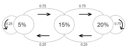
Answer: All right. When a random process is independent of previous data, we call it a Markov process. See link an example of one such process to the image to the right.
The store's three discount balances are 5%, 15%, and 20%. New custo-mers will start with a 5% discount. When they then buy something within a week, they move up one level or stay at the highest level. When they don't buy anything for the next week, they move to a lower level or stay at the lowest level. The probability that a customer buys something per week is 0.75, and, therefore, that he buys nothing is 0.25. It is a Markov process from the picture.
1. The columns of the corresponding matrix of this process are probability distributions, with elements A = (αij) index i, j ∈ {1, 2, 3}:
\[ A = \begin{pmatrix} \frac14 & \frac14 & 0 \\ \frac34 & 0 & \frac14 \\ 0 &\frac34 & \frac34 \end{pmatrix}. \]Here α21 = 3/4 means the conditional probability Pr(15%|5%), of the customer switching from a discount of 5% to 15%, while α22 = 0 is Pr(15%|15%) the pro-bability that the buyer of the 15% discount will stay at the same level discount, and α23 = 3/4 is the probability that the customer keeps the highest discount.
2. The same process, from the picture, can be viewed in the following way. Let pij(t1, t2) the probability that the customer from time (week) s and discount level j will switch to discount level i into the time r. Then let's say from the level j = 2, i.e. with a discount of 15%, can reach the level i = 1 and a discount of 5%, by going from the second to the first through each of the three levels in one of the inter-weeks m. So:
pij(s, r) = pi1(s, m)⋅p1j(m, r) + pi2(s, m)⋅p2j(m, r) + pi3(s, m)⋅p3j(m, r)
the probability of moving from the jth to the ith discount level from week s to r but over the interweek m. This is an example of the Chapman-Kolmogorov Equation. In doing so, weeks are taken in steps s < m < r.
3. Let us generalize this to the homogeneous Markov chain X0, X1, ..., Xn, ... of the state space {1, 2, ..., N}. We are looking for conditional probabilities, which is P(Xn = j | X0 = i), that the zero link of the chain will pass in n steps from i to j-th state. The states are, for example, the points at which a member of the Markov sequence is found in the nth step. For this reason, let's recall the calculus of probability:
\[ \Pr(AB | C) = \Pr(A|BC) \cdot \Pr(B|C) = \frac{\Pr(ABC)}{\Pr(BC)}\cdot\frac{\Pr(BC)}{\Pr(C)} = \frac{\Pr(ABC)}{\Pr(C)}. \]As we know, these products of AB events mean intersections of sets A ∩ B, or the conjunction A ∧ B. Thus we find the conditional probabilities:
\[ \Pr(X_2 = j | X_0 = i) = \sum_{k=1}^N \Pr(X_2 = j \wedge X_1 = k | X_0 = i) = \] \[ = \sum_{k=1}^N \Pr(X_2 = j | X_1 = k \wedge X_0 = i) \cdot \Pr(X_1 = k | X_0 = i). \]At the same time, Markov property says that in order to predict the behavior of the system in the future, it is enough to consider only the current state of the system, that the past history is not important, so the event X0 = i in the first probability does not matter. This result becomes the sum of the proba-bilities:
\[ \Pr(X_2 = j | X_0 = i) = \sum_{l = 1}^n \alpha_{l j}\cdot \alpha_{i l}, \]and it is the term, the entry of the square of the Markov matrix A² = (αij)².
4. Furthermore, it can be proved by the method of mathematical induction that:
Pr(Xn = j | X0 = i)
is the matrix element of An, i.e., the n degree of the Markov matrix A = (αij). At the same time:
\[ \Pr(X_{n+m} = i | X_0 = i) = \sum_{l=1}^N \Pr(X_{n+m} = i | X_m = l)\cdot \Pr(X_m = l | X_0 = j) \]are the Chapman-Kolmogorov equations. Probability increment Pr(Xn+1 | Xn) at one step, changes of one degree from An to An+1 are in the previous answer mentioned the speed of signal change in nth moment. Seen in this way, that discrete equation will become a Kolmogorov differential equation.
Conception » srb
Question: All right. This is a great explanation of the Chapman-Kolmogorov equations to me. However, what do they have to do with the information theory you are dealing with?
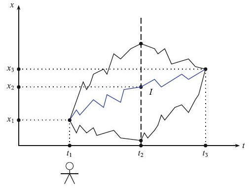
Answer: This is the easy part. First, let's try to understand what confu-ses the reader in the question posed in the image link on the left. So let's take a look at the answer from that attachment, then see my informatic explanation.
1. I will recount the first two. In short, at time t1, we have settings x1, as in the picture on the left, so whatever development they go th-rough, over t2 ∈ (t1, t3), will arrive in the same settings x3 when the time t3 comes. That is, the result includes all possible previous paths, so the process behaves just like someone without memory. It is in the previous answer Markov Property, or:
\[ \Pr(x_3, t_3 | x_1, t_1) = \sum_{x_2} \Pr(x_3, t_3 | x_2, t_2) \Pr(x_2, t_2 | x_1, t_1). \]written by probabilities in the form of Chapman-Kolmogorov equations.
Note my addition: "Whatever development they go with..." boils down to "process without memory.". In other words, if the result is the sublimation of all freedoms, or a consequence that includes all possible paths of developme-nt, then there were no freedoms. Whatever we choose, we come to the same thing.
2. The specificity of my interpretation of information theory is "reality," which is a perceptible, permanent, and true phenomenon. The mentioned equations interpret phenomena without memory, so even though they themselves are "real," what they analyze are "fictions" (unrealities that we think exist). An ongoing process has a past, and if it does not exist, even if it is true and noti-ceable, it is not reality in the aforementioned sense.
When we place such a process in reality, it degenerates. It is paradoxical when we treat the real, in real conditions, as unrealistic. Then, as a good, first of all, accurate treatment, it will find the unsustainability of the subject phenomenon in the sense of disappearing, or its permanent change, or turning those forms into some stable ones. The result will not escape the principle of minimalism. This is also the basic difference between, say, a statistical ensemble (a gas par-ticle whose entropy increases) and individual molecules (which move random-ly, not caring about the entropy change).
3. When the Markov matrix is like the above A, (Transitions, 1) isometric; it is in case det(A) = ±1, then it represents a process that does not remember even though it lasts (it is remembered by the environment); then there is no dege-neracy mentioned. In all other cases, -1 < det(A) < +1, An → 0, when n → ∞, i.e., that an infinitely long Markov chain transmission inevitably loses the initial information. That chain becomes a "black box," a transmitter whose output message tells us nothing about the input.
This also follows from direct algebra, that processes whose determinants are zero are not reversible, and that those determinants |det(A)| ≠ 1. The latter are, for example, stochastic (Markovian) processes that can go forward but not backward, although they can transmit some information. I will demonstrate this by solving the aforementioned matrix.
4. From the second column of the determinant of the matrix A, let's subtract the first one and develop the resulting determinant by the first row:
\[ \det(A) = \begin{vmatrix} \frac14 & \frac14 & 0 \\ \frac34 & 0 & \frac14 \\ 0 & \frac34 & \frac34 \end{vmatrix} = \begin{vmatrix} \frac14 & 0 & 0 \\ \frac34 & -\frac34 & \frac14 \\ 0 & \frac34 & \frac34 \end{vmatrix} = \] \[ = \frac14\begin{vmatrix} -\frac34 & \frac14 \\ \frac34 & \frac34 \end{vmatrix} = \frac14( -\frac{9}{16} - \frac{3}{16}) = -\frac{3}{16} = -0,1875. \]So -1 < det(A) < +1, so we have some information transfer, but not a reversible stochastic process. Namely, the inverse matrix of this is:
\[ A^{-1} = \begin{pmatrix} 1 & 1 & -\frac13 \\ 3 & -1 & \frac13 \\ -3 & 1 & 1 \end{pmatrix}, \]which is easy to check by direct multiplication when the unit matrix is obtai-ned AA-1 = A-1A = I. So, from the output q = Ap, we can estimate the input p, but the inverse matrix A-1 is not stochastic; there is no process A-1: q → p.
By scaling, An → A*, when n → ∞, we find:
\[ A^* = \begin{pmatrix} 0.07692308 & 0.07692308 & 0.07692308 \\ 0.23076923 & 0.23076923 & 0.23076923 \\ 0.69230769 & 0.69230769 & 0.69230769 \end{pmatrix}. \]That this is correct is easily checked with AA* = A*A = A*. The determinant of this matrix has equal rows, meaning its value is zero. The zero determinant matrix has no inverse matrix. This multiplied by any distribution probability vector (x + y + z = 1) gives:
\[ \begin{pmatrix} 0.07692308 & 0.07692308 & 0.07692308 \\ 0.23076923 & 0.23076923 & 0.23076923 \\ 0.69230769 & 0.69230769 & 0.69230769 \end{pmatrix} \begin{pmatrix} x \\ y \\ z \end{pmatrix} = \begin{pmatrix} 0.07692308 \\ 0.23076923 \\ 0.69230769 \end{pmatrix}. \]Therefore A* is a black box.
Null Space II » srb
Question: What is the null space of a stochastic matrix?
Answer: Stochastic matrices do not have "null spaces" in the set of pro-bability distribution vectors.
Namely, any square matrix A = (αij) of non-negative elements (αij ≥ 0) sums one of any column (∑i αij = 1) is stochastic. The columns of the stochastic matrix denote probabi-lity distributions. If we multiply the distribution by that matrix, the result is another distribution.
1. The zero space (Domains) of a matrix consists of the vectors that the matrix translates into zero vectors. If Ma = 0, then a will be the zero-space vector of the matrix M. For example:
\[ \begin{pmatrix} 3 & -1 & 1 \\ -1 & 1 & 1 \end{pmatrix} \begin{pmatrix} 1 \\ 2 \\ -1 \end{pmatrix} = \begin{pmatrix} 0 \\ 0 \end{pmatrix} \]matrix M of type 2×3 multiplies vector a (matrix of type 3×1), and this results in zero vector b (matrix of type 2×1 ). In the matrix equation Ma = b, here we have a ∈ Null(M), the vector which belongs to the null space of the matrix, and b = (0, 0), the vector that is the null vector. Thus, we distinguish zero vectors from zero space vectors.
2. The null vectors of the space depend on the matrix and may or may not be null vectors. In the case of the (stochastic) matrix from the previous answer:
\[ A = \frac14\begin{pmatrix} 1 & 1 & 0 \\ 3 & 0 & 1 \\ 0 & 3 & 3 \end{pmatrix} \]we have the null matrix space, Null(A), which contains only one vector, that is the null vector a = (0, 0, 0). Namely, the equation:
\[ \frac14\begin{pmatrix} 1 & 1 & 0 \\ 3 & 0 & 1 \\ 0 & 3 & 3 \end{pmatrix} \begin{pmatrix} x \\ y \\ z \end{pmatrix} = \begin{pmatrix} 0 \\ 0 \\ 0 \end{pmatrix} \]there is only one, the so-called trivial solution x = y = z = 0. Every matrix has a trivial solution and, therefore, at least one (zero vector), the element of its null space. The zero vector is a member of the null space of each matrix. Algebra easily proves that (square, regular) matrices of non-zero determinants each have only one vector of their null spaces, and these are, of course, zero vectors.
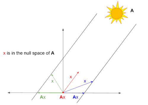
3. The physical interpretations of the zeros of the vector x of the matrix A are states (then they are the interpretations of the vector x) that the process (the interpretation of the operator A) does not change. In the picture above on the right is a link that explains it. The sun (process A) shines on objects (green, red, and blue vectors x) that cast shadows on the background (projections, vectors Ax). The one from the object that casts a shadow of zero length (red vector Ax = 0) would be from solar null space. This is a continuation of Null Space.
Null Space III » srb
Question: Да ли и докле нула простор расте са степеном матрице?
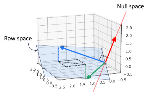
Answer: Yes, the null space can grow, but not shrink with the sca-ling of the matrix. That increase has an end.
When the process goes on and on, we formally have the matrix powe-ring:
A → A² → A³ → ..., An, ...
whose degrees affect eventual initial conditions (if such exist in the future). However, the higher the power n = 1, 2, 3, ..., the larger the null space An.
1. Theorem. Let A be a matrix of rank k ∈ ℕ (quadratic type k × k). Then, the null space of powers of A satisfies:
{0} ⊆ Null(A0) ⊆ Null(A1) ⊆ Null(A2) ⊆ ... ⊆ Null(An)
for every non-negative integer n.
Proof: Since A0 = I is a unit matrix, and 0 is the only vector mapped to the zero vector by the identity transformation, we have Null(A0) = {0}. Let vector x ∈ Null(An-1) for any natural number n ∈ ℕ. Then An-1x = 0, and when we multiply both sides by A, we get Anx = 0, which means that x ∈ An, i.e. Null(An-1) ⊆ Null(An), and that should have been proven. ∎
Interpreted, the uncertainties of reality do not grow over time. We can say that since we consider "reality" as perceptible, permanent, and true, and in the null space there are states (vectors) that disappear in the process. To put it another way, in the world around us there are "fictions" (unrealities) whose number is not decreasing. This is another confirmation of principled minimalism.
Uncertainties decrease with time, but they cannot disappear completely. This is clear from the fundamental uncertainty of natural flows. However, from the positions of null space and the previous theorem, we find the same following the next two theorems.
2. Theorem. Let A be a matrix of rank k ∈ ℕ. If there is a number n ∈ {1, 2, ...} such that Null(An) = Null(An+1), then Null(An) = Null(An + m) for each numb-er m ∈ {1, 2, 3, ...}.
Proof: It suffices to prove that from Null(An) = Null(A n+1) follows the same for a step more Null(An+1) = Null(< var>An+2) because then a chain of equa-lity is obtained, in general, Null(An) = Null(An+m) respectively for m = 1, 2, 3, ..., where we know that Null(An) ⊆ Null(An+m) from the previous theorem.
Since An+2x = 0 means A n+1Ax = 0, that is the vector Ax ∈ Null(An+1). Howe-ver, by assumption, Null(An) = Null(An+1), so Ax ∈ Null(An), i.e. AnAx = 0, i.e. An+1x = 0, so x ∈ Null(An+1).
Therefore, all terms from Null(An+2) also belong to Null(An+1). Now we also have the inclusion Null(An+2) ⊆ Null(An+1) which, with the previous one, becomes equal to Null(An +2) = Null(An+1). Hence the required assertion by induction. ∎
Stopping the growth of null space certainly occurs, because not all uncer-tainties can be canceled. In fact, the following theorem talks about it.
3. Theorem. Let A be a matrix of rank k ∈ ℕ. Then Null(Ak) = Null(Ak+1).
Доказ: From the previous two theorems, Null(Ak) = Null(Ak+1), because the dimension of the matrix A is not greater than its rank k, and thus neither the number of base vectors in general nor the number of independent vectors of its null space. ∎
Row Space » srb
Question: What is the row (column) space of a matrix?
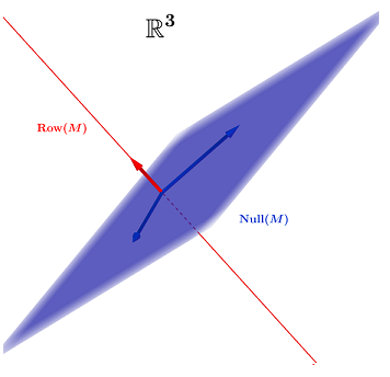
Answer: There are four basic subs-paces of matrices: i row spaces and ii column spaces, iii null space, and iv transposed null space (left null space). Let's look at their meanings, interpretations, and reasons for some verticals.
1. The column space (also rows) of a matrix A of type m×n is the vector space that spans those columns. For example, the three columns of the matrix:
\[ A_{2\times 3} = \begin{pmatrix} 1 & 2 & 3 \\ 0 & -1 & 1 \end{pmatrix} \]span the 2-dimensional space of the basis of any two of its three columns and any two independent 2-component vectors. However, the types of this matrix are again independent vectors, but they are two 3-component vectors. Given vectors, say v1 and v2, form linear combinations u = av1 + bv2 with arbitrary real (complex) numbers a and b, the space spanned by the given vectors. The null space of this matrix would belong, for example, has vector w = (-5, 1, 1)⊤, because:
\[ A\mathbf{w} = \begin{pmatrix} 1 & 2 & 3 \\ 0 & -1 & 1 \end{pmatrix} \begin{pmatrix} -5 \\ 1 \\ 1 \end{pmatrix} = \begin{pmatrix} 0 \\ 0 \\ 0 \end{pmatrix} = 0. \]Obviously, the rows of the matrix are perpendicular to the vectors of its null space. And the "left null space" is created by transposing and multiplying the vectors to the left of the matrix.
2. Example. Are the following vectors in the null space of the given matrix:
\[ \mathbf{u} = \begin{pmatrix} -5 \\ 1 \\ 7 \end{pmatrix}, \quad \mathbf{v} = \begin{pmatrix} 1 \\ -2 \\ 3 \end{pmatrix}, \quad A = \begin{pmatrix} 2 & 3 & 1 \\ -3 & -1 & -2 \\ 0 & 7 & -1 \end{pmatrix}. \]Check if they are perpendicular to the vectors of its rows (columns).
Solution: By multiplying, we find Au = (0, 0, 0)⊤ and Av = (-1, -3, -17)⊤. In other words, u ∈ Null(A) and v ∉ Null(A). This means that the rows of the matrix are perpendicular to the vector u, but not to the vector v. Matrix col-umns are not like that. By transposition, we get the equations u⊤A⊤ = (0, 0, 0) and v⊤A⊤ = (-1, -3, -17), so this verticality passes from the rows on columns. ∎
3. The determinant of the example matrix is zero, det(A) = 0. Only two of its three rows (columns) are linearly independent vectors. Hence there is exactly one non-trivial vector in the null space of dimension dim Null(A) = 1, so that with the two dimensions of the space spanned by its rows (columns), there would be a total of three dimensions, i.e., the order of the matrix (type 3×3).
From the above, the system of linear equations Ax = b has (at least one) solution if and only if the vector b is in the space spanned by the columns of matrix A. It is a well-known item of algebra, and I do not state it as a peculi-arity. And, that the higher power of the matrix has a smaller column space — we know less often, and it is worth more for the next information theory.
4. Theorem. Let X be the space of all k×1 columns of matrix A of type k×k. Then for the column space of the powers of the matrix:
X = Col(A0) ⊇ Col(A1) ⊇ Col(A2) ⊇ ... ⊇ Col(An)
for any natural number n ∈ ℕ.
Proof: Since A0 = I, that x = A0x for each x ∈ X. Therefore, Col(A0) = X. For an arbitrary natural number n let x ∈ Col(An). Then, by definition of column spa-ce, there is y ∈ X such that Any = x, which can be written A n-1(Ay) = x. Hence x ∈ Col(An-1). Therefore, all members of Col(An) are in Col(An- 1), or to say in other words Col(An-1) ⊇ Col(An). ∎
The space of the columns decreases exactly as much as the zero-space incr-eases by scaling the matrix so that the sum of the dimensions of one and the other always remains the same, equal to the order of the given matrix. In the previous interpretation, here during the process, An when n → ∞, is about supplementing reality with fiction. In the case of the Markov chain, when by stringing the number of links, it tends to a black box and only one independe-nt column (row) vector, the limit value is a continuous constant duration that is not affected by the initial messages.
5. Looking more broadly, including the vast scale of the universe, we do not always have repetitions of the same processes or powers of constant matrices. It is also impossible due to the equivalence of truths and falsehoods (bijections replacing "true" with "false" in expressions of algebraic logic). It is impossible to reduce the total amount of true statements (reality) without an equal decre-ase in untruths (fiction). The way out of this paradox, among other things, is in changes both in the process generators themselves and in what they are processing.
Such an "exit" is especially in the spirit of this theory of information, where we work with information as a structure of space, time, and matter, the essence of which is uncertainty. The future flows towards a more likely, less informative, i.e., more certain and orderly, calmer, and perhaps more efficient, but also less imaginative. It is like reality that it lasts and has an ever-longer past (also informative), a residue that directs and limits its ongoing present.
Row and Column » srb
Question: Why do you think the row and column spaces of a matrix have the same dimensions?
Answer: It's not "my discovery"; it's a long-established fact of linear alg-ebra (Rang). Here are some more details about it.
1. The matrix A of type m×n will have m rows, and n columns. Let these be k-dimensional vectors. Certainly k ≤ max{m, n}.
So there is base E = {e1, e2, .. ., ek} of k vectors, ei respectively i = 1, 2, ..., k, which span the column space Col(A) of matrix A. The columns are linear combinations of the vectors of that basis. Let's form the matrix B[e1, e2, ..., ek] whose columns are base vectors E. Then A = BC, where C is the matrix of columns which are the coordinates of the columns of A represented by the base E.
Similarly, multiplication of transposed A = C'B', where B'[e'1, e'2, ..., e'k] is matrix with rows vectors e'j bases E' in which every vector row of matrix A can be written. The base E' span the space Row(A) of the rows matrix A, and the rows of the matrix C' are the coefficients of those developments.
The base E cannot have more vectors than its components, than n, more pre-cisely than the rank of the base of the rows of the matrix A. Hence, we have dim Col(A) ≤ dim Row(A). However, the reverse is also true: the base E' has no more vectors than its components, no more than m, or more precisely, no more than the rank of the column base of the matrix A, and hence we have dim Row(A) ≤ dim Col(A). These two inequalities show that the row and column spaces have the same dimensions.
In both cases, multiplication gives the same matrix A, linear transformations of all vectors on which A acts lead to the same results, so the bases of such spaces are of the same dimension, dim Col(A) = dim Row(A). Note that this does not mean that the basis vectors E and E' are equal.
2. Example. A type m×n (2×3) matrix is given:
\[ A = \begin{pmatrix} 1 & 2 & 3 \\ 2 & 1 & 0 \end{pmatrix}. \]Let's write some bases and corresponding matrices from (1).
Solution: For the columns of matrix A we have in turn:
\[ E: \quad \mathbf{e}_1 = \begin{pmatrix} 1 \\ 0 \end{pmatrix}, \quad \mathbf{e}_2 = \begin{pmatrix} 0 \\ 1 \end{pmatrix}, \quad B = \begin{pmatrix} 1 & 0 \\ 0 & 1 \end{pmatrix}, \] \[ \begin{pmatrix} 1 \\ 2 \end{pmatrix} = 1\cdot \mathbf{e}_1 + 2\cdot \mathbf{e}_2, \quad \begin{pmatrix} 2 \\ 1 \end{pmatrix} = 2\cdot \mathbf{e}_1 + 1\cdot \mathbf{e}_2, \quad \begin{pmatrix} 3 \\ 0 \end{pmatrix} = 3\cdot \mathbf{e}_1 + 0\cdot \mathbf{e}_2, \]so C = A and A = BC. In the case of matrix types A we find:
\[ E': \quad \mathbf{e}'_1 = \begin{pmatrix} 1 & 1 & 1 \end{pmatrix}, \quad \mathbf{e}'_2 = \begin{pmatrix} 0 & 1 & 2 \end{pmatrix}, \quad B' = \begin{pmatrix} 1 & 1 & 1 \\ 0 & 1 & 2 \end{pmatrix}, \] \[ \begin{pmatrix} 1 & 2 & 3 \end{pmatrix} = \mathbf{e}'_1 + \mathbf{e}'_2, \quad \begin{pmatrix} 2 & 1 & 0 \end{pmatrix} = 2\mathbf{e}'_1 - \mathbf{e}'_2, \] \[ C' = \begin{pmatrix} 1 & 1 \\ 2 & -1 \end{pmatrix}. \]By multiplying matrices, we now easily check A = C'B'. ∎
3. In this theory, the subject does not perceive the object as it is, but it's dual reality. Each subject is thus unique. If we have subject state x = (x1, ..., xn) and possible observation states y = (y1, ..., yn) they mean vectors, sequences of the same length n = 1, 2, 3, ... and different variances. So the perception of infor-mation is:
\[ \mathbf{x}^\top \mathbf{y} = \begin{pmatrix} x_1 & \cdots & x_n \end{pmatrix} \begin{pmatrix} y_1 \\ \vdots \\ y_n \end{pmatrix} = x_1y_1 + \cdots + x_ny_n. \]This can be written:
\[ \mathbf{x}^\top y = (A^\top u)^\top y = u^\top A y = u^\top (Ay) = u^\top v, \]which means that the perception of the first x is equal to the perception of some other subject u, now the object v = Ay, then a different one, and the same y changed by some mapping A. By transposing the columns, we change the types and vice versa, and the dimensions of the perceptions remain the same, although the number of their elements does not have to be the same (m ≠ n) when the matrix (A) is not square.
We know that not all biological species have the same senses. Vision is impo-rtant for birds, sound for bats, and smell for forest animals, but even when they have the same senses, animals do not perceive the same colors of light or frequencies of sound and chemicals. Of course, there are many more such senses, that is, ways of communicating with the environment, or interactions. That's why the mentioned matrix does not have to be square, but those belonging to subjects and objects are parts of the same reality with the same number of dimensions.
Column Space » srb
Question: Do you have something more to add about the column space?
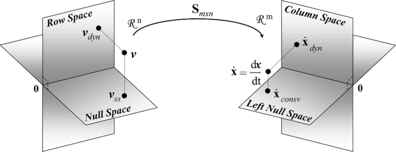
Answer: In linear algebra, the column space (also named domain or image) of a matrix A is the span (of all linear combinations) of its column vectors. As is Col(A) perpendicular to the null space Null(A) of that matrix so is the transpo-sed row space Row(A) also perpendicular to the transposed null space of the same matrix. However, these are known things and I believe you expect me to find out something unknown to others. Let's first look a couple of well-known algebra statements that establish the preceding more directly.
1. Theorem. Let A be a matrix of type k×k. If there exists some n = 1, 2, 3, ..., a natural number such that Col(An) = Col(An+1), then Col(An) = Col( An+m) for every natural number m.
Proof: It suffices to prove that from Col(An) = Col(A n+1) yields the following Col(An+1) = Col(An+2), because the required statement then follows by indu-ction. By now we know (Row Space, Theorem 4) that Col(An+1) ⊇ Col(An+2), and we need inclusion in the other direction.
Let X be the space of all columns of the vector k×1. Let's take an arbitrary x ∈ X and let u = Anx. By definition in ∈ Col(An), then from Col(An) = Col(An+1) followed by u ∈ Col(An+1). Thus, there is y ∈ X that u = An+1y, or u = An(Ay). The two give Anx = An(Ay). Therefore, we proved that behind every x ∈ X is some y ∈ X, so just found is valid.
Further, suppose u ∈ Col(An+1). Then there is x ∈ X such that An+1x = u, or AAnx = u. From the above, there is y ∈ X that AAnx = AAn(Ay) = An+2y = u. Said differently, we got u ∈ Col(An+2). This means that all members from Col(An+1) are also in Col(An+2), and Col(An+1) ⊆ Col(An+2). This concludes the proof. ∎
The column space by powering the A matrix decreases (more precisely, it does not increase), and its null space increases (does not decrease). If by some pow-er n ∈ ℕ there is a stoppage in that decline, the tendency of decline stops alto-gether. Let's check that such a deadlock is definitely happening.
The decrease of column space, by successive mappings of A, A², A³, ... ends with the same exponent as the growth of zero space of this matrix, because the sum of their dimensions, the first and second, is equal to the rank (number of dimensions) of that matrix. This was established in another way in the previo-us answers. I surround so much to make the transition from this abstraction to its interpretation in information theory more believable, to the paradox that then gets an interesting outcome.
3. An ongoing process, An with increasing exponent n, spontaneously produ-ces more certain states. In doing so, I interpret the column space as "real" in contrast to the null space, which would be "fictitious" (Null Space). It is absu-rd to reduce the first at the expense of the second, considering their equivale-nce, looking more broadly. But, in the example of energy changes, we know about various local disturbances of the balance during its global keeping. I've mentioned it before, and it's not new enough to answer here.
First, let's understand that we add the speed of the boat sliding on the water to the speed of the flowing water to get the speed of the boat relative to the shore. Then, this also applies to velocities as directed lengths whose "sum" is the dia-gonal of the parallelogram to which they are sides. I'm talking about the gene-ralization to vectors and the idea of a vector space that has only four axioms and includes the addition of forces, momentums, polynomials, solutions of differential equations, and states in quantum mechanics, and who knows what else.
Similarly, the theory of probability matured, from Pascal's sporadic and disconnected, but orderly solutions (16th century), until Kolmogorov's three axioms (1933), with which he translated that theory into a rounded whole. This way of generalization, translated into physical reality and billions of years of development of the cosmos that spontaneously leads to greater certainty (according to this information theory), would make there be more order and fewer fragmented correct theories. Simply, if they were produced by a smaller number of principles.
In this way, there would be more truths, order, and rules, with fewer and fewer theories. The fantasy space would appear larger locally, due to more combinations, with actually shrinking globally. As in the "big number" cases of probability theory, we would encounter different solutions for the small world and the big world.
Enlarging » srb
Question: On what basis do you stand the hypothesis of a decrease in the speed of light in a vacuum with the aging of the universe?
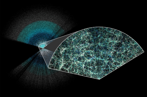
Answer: Yes, it's still just a working hypothesis. However, I have it in a package with maturations due to principled minimalism. The same applies to space. Spontaneously, it tends equally towards more proba-ble states, not informative, and mo-re certain ones. It is too extensive to list all the reasons, out of the many that I have already stated, so here is just one that I haven't men-tioned (for a long time).
1. The law of large numbers inspires. When moving from few to many outco-mes, it makes randomness turn into regularity. This "unusual" phenomenon, placed in an abstract probability space along with a metric, should be like the slow-motion of the celestial bodies of the galaxy in relation to the motions of the electrons in the atom — when we place them in the same frame. It takes about a hundred thousand years for light to travel from one end of our galaxy to the other, and only a fraction of a second for an electron to travel the length of an atom.
That macro world of galaxies becomes a kind of physics of a smaller world in which the speed of light in a vacuum would decrease; if instead of the current 300,000 km/s we reduce it to, say, about 30 km/s, but not only in plasmas as consistently in all natural legalities.
2. When we consistently decrease the speed of light in all the laws of physics, then we will take care that the product of the photon's wavelength and frequ-ency, λf = c, also decreases proportionally by, say, a hundred times. This can easily mean reducing all the dimensions of the micro world so that we get the same physics again, except that we put ourselves in the position of something bigger; that is, everything else is smaller. We would find ourselves in the posi-tion of comparative observers who will experience their own times equally in both relative motion systems.
The present would behave like a body falling into a black hole from the per-spective of an observer outside of gravity, that is, from the distant past. That would be a slowing down of event frequencies and, correspondingly, smaller amounts of outcomes and less information. The big question is whether it would then give not only a more peaceful but also a more certain world.
3. We have confirmation of the described acceleration of light, for now, only in the distant past of the universe at the time of its cosmic inflation. At that time, the boundary of space expanded faster than light, but we are not entirely sure whether the eventual particles of space at that time could move at those incr-eased speeds, nor whether the theory of inflation is reliable (it is official phy-sics, but many were like that before disputes).
The law of large numbers also warns us that this need not be a simple homo-thety. For example, the illusion of an expanding universe (Universe II), with which this idea begins, would, due to our ever-decreasing units of length, actually give the increasing mean distance between galaxies and the bound-aries of the universe (visible and otherwise). This would imply an increasing past, then duration, and then "reality" of the cosmos in the manner of my definition.
The actual receding of galaxies means a thinning of the substance of the universe and a decrease in the density of information of the present. This is consistent with the principle of minimalism, but also with the slowing down of time of masses between which the space escapes more quickly into the future. However, some noticeable, more easily measurable differences in the speed of light in a vacuum now and then would only occur at very large distances, as in the case of time dilation visible only for speeds close to the speed of light.
Diagonal » srb
Question: That story about the universe is sad and gloomy. I find that kind of universe depressing, don't you think so?
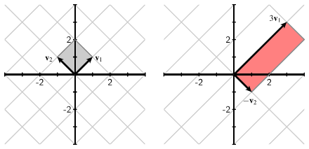
Answer: You say we are prisoners of a cosmic "illusion" and confined within us is the only such space-time, but is this 13.8 billion years not enough?
This is a detail from a conversation I often have, as I try to explain the more exciting aspects of algebra and their interpretation. That, a more interesting part of the conversation, we had about finding the powers of a matrix and terminating such in "black boxes" of processes in general (not just Markovian ones).
1. The link in the image above on the left leads to a matrix with two eigen-vectors:
\[ A = \begin{pmatrix} 1 & 2 \\ 2 & 1 \end{pmatrix}, \quad v_1 = \begin{pmatrix} 1 & 1 \end{pmatrix}, \quad v_2 = \begin{pmatrix} -1 \\ 1 \end{pmatrix}, \]with eigenvalues λ1 = 3 and λ2 = -1, so the eigen, i.e. characteristic equation Avk = λkvk holds for both indices k ∈ {1, 2}. It is easy to check by multiplica-tion, but it is not so easy to find these numbers (λ) or vectors (v). However, once we have them, we also have the equation:
\[ \begin{pmatrix} 1 & 2 \\ 2 & 1 \end{pmatrix} = \begin{pmatrix} 1 & -1 \\ 1 & 1 \end{pmatrix} \begin{pmatrix} 3 & 0 \\ 0 & -1 \end{pmatrix} \begin{pmatrix} 1/2 & 1/2 \\ -1/2 & 1/2 \end{pmatrix}, \]that is, A = PDP-1, where P[v1, v2] is a matrix whose columns are eigenvectors, and P-1 is its inverse matrix. The matrix D is diagonal which on the main dia-gonal has the eigenvectors of the matrix A respectively. Study this, and let's move on.
2. Starting from A = PDP-1, by exponentiation we find:
A² = (PDP-1)² = (PDP-1)(PDP-1) = PD(P-1P)DP-1 = PD²P-1,
A³ = A²A = PD²P-1 PDP-1 = PD³P-1,
An = PDnP-1, n = 0, 1, 2, 3, ...,
\[ \begin{pmatrix} 1 & 2 \\ 2 & 1 \end{pmatrix}^n = \begin{pmatrix} 1 & -1 \\ 1 & 1 \end{pmatrix} \begin{pmatrix} 3^n & 0 \\ 0 & (-1)^n \end{pmatrix} \begin{pmatrix} 1/2 & 1/2 \\ -1/2 & 1/2 \end{pmatrix}, \] \[ A^n = \frac12\begin{pmatrix} 3^n + (-1)^n & 3^n - (-1)^n \\ 3^n - (-1)^n & 3^n + (-1)^n \end{pmatrix}. \]This is one way of finding the powers of a matrix, by diagonalization.
3. When we consider matrix exponentiation as a process and extract, say, the common factor 3n of this matrix exponent, we get An = 3nBn, where the seco-nd factor gives the matrix:
\[ B_n \to B = \begin{pmatrix} 1/2 & 1/2 \\ 1/2 & 1/2 \end{pmatrix}, \quad n \to \infty. \]This boundary, B, is a stochastic matrix and a “black box” interpreted as a dis-tribution transmitter. It maps all (binary) distributions into the same homoge-neous (1/2, 1/2). Its copies do not reveal the originals. In other words, a proce-ss that would be presented in this way, at the output of a long power-up, wou-ld give a fake message that there was some impersonality at the input, like the cosmic mush of the early stages of the Big Bang.
4.Theorems on column space (up to Column Space) speak of this narrowing of the column space of an exponent matrix, regardless of whether it has real or complex coefficients. In this way, Markov chains, quantum processes, or real (macro-world) ones, which I often take as an example here, will converge to the "black box.". Reducing the dimensions of the column space by exponenti-ating the matrix means its convergence towards equal columns, which gives the observer at the end of the chain (from the present) a "false" image of an impersonal distant past.
In this sense, we are prisoners of a version of the development of the cosmos, one that could perhaps be different, but which we can only fantasize about and complain about our “gloomy” fate. However, isn’t a world with so many billio-ns of years of its duration and distance, with countless galaxies in vast expan-ses, enough for us not to feel unfree?
Degeneracy » srb
Question: What if a matrix has double eigenvalues?
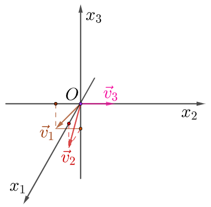
Answer: It is not always the case that a k×k matrix has all k distinct eigenvalues. The image shows such a result and has the link leading to the way for finding the eigenvalues of the λ1 = 2, λ2 = 2, and λ3 = 1 for the matrix:
\[ A = \begin{pmatrix} 2 & 0 & 0 \\ 1 & 2 & 1 \\ -1 & 0 & 1 \end{pmatrix} \]and the corresponding (vk) eigen-vectors, respectively:
\[ \begin{pmatrix} 0 \\ 1 \\ 0 \end{pmatrix}, \quad \begin{pmatrix} -1 \\ 0 \\ 1 \end{pmatrix}, \quad \begin{pmatrix} 0 \\ -1 \\ 1 \end{pmatrix}, \]so that Avk = λkvk, respectively for k = 1, 2, 3. This matrix is a linear operator that doubles the vectors v1 and v2 without changing their directions, but the vector v3 remains the same. It changes the directions and possibly intensities of all other non-zero vectors in its action space.
1. This matrix is degenerate, because it has repeated eigenvalues (λ1 = λ2) with linearly independent eigenvectors. It has eigenvectors v1, v2, and v3 that span a 3-dimensional vector space. These are the columns of the auxiliary matrix P[v1, v2, v3], or:
\[ P = \begin{pmatrix} 0 & -1 & 0 \\ 1 & 0 & -1 \\ 0 & 1 & 1 \end{pmatrix}, \quad P^{-1} = \begin{pmatrix} 1 & 1 & 1 \\ -1 & 0 & 0 & \\ 1 & 0 & 1 \end{pmatrix}. \]The latter is the inverse of the former, so the product PP-1 = P-1P = I is an identity matrix. However, A = PDP-1, where:
\[ D = \begin{pmatrix} 2 & 0 & 0 \\ 0 & 2 & 0 \\ 0 & 0 & 1 \end{pmatrix} \]diagonal matrix. Its diagonal elements are the eigenvalues of the matrix A in order, and all others are zero. By exponentiation, as in the answer above, we find An = PDnP-1, i.e. An = 2nBn with the matrix:
\[ B_n = \begin{pmatrix} 1 & 0 & 0 \\ 1 - 2^{-n} & 1 & 1 - 2^{-n} \\ -1 + 2^{-n} & 0 & 2^{-n} \end{pmatrix} \to B = \begin{pmatrix} 1 & 0 & 0 \\ 1 & 1 & 1 \\ -1 & 0 & 0 \end{pmatrix}, \quad n \to \infty. \]The limit matrix B is not stochastic, because it has negative coefficients, even though the sum of each column is one. Two of its columns are identical, and its column space is 2-dimensional, so based on the output vector y = Bx we cannot accurately determine the input x.
2. Let's imagine we have three containers with values of something (money). Process A doubles the value of the first in every step. It doubles the value of the second by adding the values of the first and third. It takes a portion of the value equal to the first from the third container.
When there are no values in the first and third containers (v1), then the pro-cess A in the subsequent steps only doubles the value of the second container, leaving the first and third at zero. A similar equilibrium exists when an equal amount is missing from the first container as there is in the third, with the second being empty (v2). All three quantities are then doubled, but their relative ratios are the same. Finally, the third eigenvector (v3) is the empty state of the value in the first container with as much in the second as there is in the third. The action A then cannot change either the ratios or the values of the containers at all.
By continually repeating the process A, it will become increasingly clear (B) that the value of the first vessel is doubled in steps such that the amounts of the second are the doubled sum of the quantities of all three. The third is the negative quantity of the first. Further, these mutual relations of the values of the vessels remain the same. When we normalize these vectors, as is implied in quantum mechanics, we ignore the coefficient 2n in front of the matrix B.
3. I try to make it easier to understand the statement of results by repeating operations with examples. In copies of copies, the originals change, but some directions survive and dominate. They impose themselves and persist as a latent force that spontaneously directs values and adapts copies to states that will no longer change. Stated this way, it is a kind of principled minimalism in the abstract form of linear algebra.
If we work with interpretations of vectors as states of physical systems and linear transformations of their processes, then we cannot stray far from the principles of minimalism. States adapt to processes, but processes are also vectors, so processes adapt to processes. The entire cosmos is being organi-zed and simplified. That's the point of the column space theorems.
Taking Over » srb
Question: Explain to me what you meant by "taking over" then?

Answer: Similar to borrowing, then (from one of the informal conversa-tions), the said "taking over" refers, to put it dramatically, to governing the cosmos by means of the excess of free will that we with vitality ha-ve in relation to the dead physical substance of which we are compos-ed. That substance follows the pri-nciple of least action, and we are much looser in minimalism with which we have an excess of will.
1. Having choices that inanimate physical matter does not have, we change our destiny, our environment, and our course. By changing states and processes that would not exist without our will, we change the universe itself. This raises several questions, one of which is: How far-reaching are such changes? Is it just scratching the surface of something much bigger, or is it like moving from one room to another entirely? Why? — will be the best piece of the answer to this question.
2. Considerations of the column space of the powers of matrices show us that processes, by repeating themselves, strive to constantly reduce the differences of previous states in order to lead them to their outcomes. They are silent op-ponents of our free will that regularly win in the long run. As if by the law of “action and reaction,” we invest our excess of choice in relation to dead physi-cal matter so that this dead world will give us a part of itself. As much as we give, we receive and nothing more.
3. On the other hand, we have the theory of deterministic chaos, which sees that there are small triggers, small actions that cumulatively reach large con-sequences. Because they are deterministic, these phenomena are not easy to influence, but they are periodic and thus become limited in scope (Attractor). The chaotic behaviors were first observed and studied in meteorological phe-nomena. One of the founders of chaos theory, Edward Lorenz (1917–2008), was a mathematician and meteorologist.
4. As in the case of lies, which attract us with their comfort (untrue, deficient information, in accordance with the principle of minimalism), then it would go towards the sobering up and disappointment of the deceived. It opens up that problem then to cover the matter now, taking over the solution from the future, and as in a zero-sum game (as much as one gains, so much the other loses) and the wolf is full and the sheep are all. When a good liar also happe-ns, then this “game of taking over” can last and last. As in such cases, the disruption of dead physical reality can cover great distances (spatial and temporal).
Transmitting itself over great distances, the distortion of truth in its steps must receive additional impulses for its continuation. Such are the processes of physical reality, by the way, when we notice that every physical information has its own effect, and if the movement of the present from the past into the future is what this information theory narrates. The spontaneous tendency towards greater probability, therefore less information, i.e. less action, is the foundation of the theory, whereby the complete absence of action is impossi-ble. However, the law of conservation and the taking over of "you get as much as you give" only came into play.
5. Similar to the described disruption of truth, vitality also rolls through living beings, their deaths and births, the transmission of hereditary traits, and the “selection of the fittest” (evolution). At this level, it is no longer just a matter of randomly selecting equally probable ones, but the principle of minimalism also goes towards the duration of life. For example, striving for freedom from information, a living individual surrenders its freedom to the collective, for example, for the sake of security. Improving efficiency is often a smaller expenditure of information (action) for the same amount of communication (interaction).
The transfer of disturbances is also the development of science, technology, and knowledge in general. When Newton was asked how he managed to dis-cover physics and gravity (1687), he replied that he stood on the shoulders of giants. Striving for order, similar to the process of granting personal freedoms to groups, dominance, and efficiency, we want lawfulness, that is, less uncer-tainty and fewer options. Taking from the future (desiring greater order then), the explorer of the unknown exposes himself to the inconvenience of more options (creativity) now.
5. Mathematics is an analogous process of merging and associating into larger logical conglomerates. This was also largely noticed by Poincaré (1854–1912), who philosophized about mathematics as the skill of merging similar images, or symbols, that is, concepts. With his skill (using lies in the search for truth), the mathematician bridges (Bridging, 6) and creates larger groups of islands of truth, otherwise inaccessible to a deductive theory that would be of truths and only truth. However, this is how nature works in developing the cosmos with principled minimalism, I suppose.
Recursion IV » srb
Question: Do you have any other way to find the n-th degree of a matrix besides diagonalization?

Answer: Yes, of course. Recursion is the typical way of finding the de-gree of a matrix. By the way, the question about recursion has often come to me (Recursion III).
1. Recursive relation:
an + αan-1 + βan-2 = 0,
has indices n = 1, 2, 3, ... which will denote the values of the variables a1, a2, a3, ..., where any two conse-cutive ones define the third. Here α and β are arbitrary constants. It has the characteristic equation with solutions x1 and x2:
x² + αx + β = 0,
\[ x_{1,2} = \frac{-\alpha \pm \sqrt{\alpha^2 - 4\beta}}{2}. \]When the solutions are different (x1 ≠ x2), the general solution of the given recursion is:
an = c1x1n + c2x2n,
where c1 and c2 are unknown constants defined by the initial conditions. If the characteristic equation has a double solution (x1 = x2 = x0), then the general solution of the given recursive relation is:
an = c1x0n + c2nx0n,
where again c1 and c2 are constants determined by the initial conditions.
These are indeed solutions to the given recursive relation, which is easily verified by substitution. For example, when the roots of the characteristic equation are distinct (x1 ≠ x2), we have:
an + αan-1 + βan-2 =
\[ (c_1x_1^{n+1} + c_2x_2^{n+1}) + \alpha(c_1x_1^n + c_2x_2^n) + \beta(c_1x_1^{n-1} + c_2x_2^{n-1}) = \] \[ = c_1(x_1^{n+1} + \alpha x_1^n + \beta x_1^{n-1}) + c_2(x_2^{n+1} + \alpha x_2^n + \beta x_2^{n-1}) \] \[ = c_1x_1^{n-1}(x_1^2 + \alpha x_1 + \beta) + c_2x_2^{n-1}(x_2^2 + \alpha x_2 + \beta) = 0. \]Similarly, the double solution is checked (x1 = x2).
2. The same recursive relation (m = n - 2) can be written as a matrix:
\[ a_{m+2} = \begin{pmatrix} 0 & 1 \end{pmatrix} \begin{pmatrix} 0 & 1 \\ -\beta & -\alpha \end{pmatrix}^m \begin{pmatrix} a_1 \\ a_2 \end{pmatrix}. \]Namely, for m = 1, we check:
\[ \begin{pmatrix} 0 & 1 \end{pmatrix} \begin{pmatrix} 0 & 1 \\ -\beta & -\alpha \end{pmatrix} \begin{pmatrix} a_1 \\ a_2 \end{pmatrix} = \begin{pmatrix} -\beta & -\alpha \end{pmatrix} \begin{pmatrix} a_1 \\ a_2 \end{pmatrix} = a_3, \]and hence -βa1 - αa2 = a3, i.e. the above relation for m = 2. Next step:
\[ \begin{pmatrix} 0 & 1 \end{pmatrix} \begin{pmatrix} 0 & 1 \\ -\beta & -\alpha \end{pmatrix}^2 \begin{pmatrix} a_1 \\ a_2 \end{pmatrix} = \] \[ = [\begin{pmatrix} 0 & 1 \end{pmatrix} \begin{pmatrix} 0 & 1 \\ -\beta & -\alpha \end{pmatrix}][\begin{pmatrix} 0 & 1 \\ -\beta & -\alpha \end{pmatrix} \begin{pmatrix} a_1 \\ a_2 \end{pmatrix}] \] \[ = \begin{pmatrix} -\beta & -\alpha \end{pmatrix} \begin{pmatrix} a_2 \\ a_3 \end{pmatrix} \]that is -βa2 - αa3 = a4, which gives the above recursive relation for m = 3. Further checks follow by induction. The proof by mathematical induction follows from:
\[ \begin{pmatrix} 0 & 1 \end{pmatrix} \begin{pmatrix} 0 & 1 \\ -\beta & -\alpha \end{pmatrix}^m \begin{pmatrix} a_1 \\ a_2 \end{pmatrix} = \] \[ = [\begin{pmatrix} 0 & 1 \end{pmatrix} \begin{pmatrix} 0 & 1 \\ -\beta & -\alpha \end{pmatrix}] [\begin{pmatrix} 0 & 1 \\ -\beta & -\alpha \end{pmatrix}^{m-1} \begin{pmatrix} a_1 \\ a_2 \end{pmatrix}] \] \[ = \begin{pmatrix} -\beta & -\alpha \end{pmatrix} \begin{pmatrix} a_m \\ a_{m+1} \end{pmatrix} = a_{m+2}, \]where the induction assumption is in the second square bracket.
3. Example. Find the general solution of the recursion:
an = 2an-1 - an-2,
with the initial conditions a1 = -1 and a2 = 1.
Solution: First way. The characteristic equation is x² - 2x + 1 = 0, with a double solution x0 = 1. From (1) the general solution is an = c1 + nc2, so including the initial conditions from the system of linear equations:
a1 = c1 + c2 = -1, c1 + 2c2 = 1,
we find c1 = -3 and c2 = 2, and hence the required recursion an = -3 + 2n. This is a sequence of numbers: a1 = -1, a2 = 1, a3 = 3, a4 = 5, a5 = 7, ...
Second way. Since α = -2 and β = 1, it will be:
\[ a_{m+2} = \begin{pmatrix} 0 & 1 \end{pmatrix} \begin{pmatrix} 0 & 1 \\ -1 & 2 \end{pmatrix}^m \begin{pmatrix} -1 \\ 1 \end{pmatrix}, \]where we have included the initial values in the column matrix (vector). Hence:
\[ a_{m+2} = \begin{pmatrix} 0 & 1 \end{pmatrix} \begin{pmatrix} -m + 1 & m \\ -m & m + 1 \end{pmatrix} \begin{pmatrix} -1 \\ 1 \end{pmatrix} = 2m + 1. \]Substituting m = n - 2, it is the previously found recursion, and the same searched string is obtained. ∎
4. Let's find the mth power of the second-order matrix. Then:
\[ M^{m+1} = \begin{pmatrix} a_{m+1} & b_{m+1} \\ c_{m+1} & d_{m+1} \end{pmatrix} = \begin{pmatrix} a & b \\ c & d \end{pmatrix}^{m+1} = \] \[ = \begin{pmatrix} a & b \\ c & d \end{pmatrix} \begin{pmatrix} a & b \\ c & d \end{pmatrix}^m = \begin{pmatrix} aa_m + bc_m & ab_m + bd_m \\ ca_m + dc_n & cb_m + dd_m \end{pmatrix}, \] \[ \begin{cases} a_{m+1} = aa_m + bc_m & b_{m+1} = ab_m + bd_m \\ c_{m+1} = ca_m + dc_n & d_{m+1} = cb_m + dd_m \end{cases} \]From the first and third of these four equations we find:
\[ a_{m+1} = aa_m + bc_m, \quad c_{m+1} = ca_m + dc_m, \] \[ a_{m+2} = aa_{m+1} + bc_{m+1} = aa_{m+1} + b(ca_m + dc_m) = \] \[ = aa_{m+1} + bca_m + d(a_{m+1} - aa_m) \] \[ = aa_{m+1} + bca_m + da_{m+1} - ada_m. \]By a similar procedure and arrangement, then shifting m = n - 2 we obtain:
an - (a + d)an-1 + (ad - bc)an-2 = 0,
bn - (a + d)bn-1 + (ad - bc)bn-2 = 0,
cn - (a + d)cn-1 + (ad - bc)cn-2 = 0,
dn - (a + d)dn-1 + (ad - bc)dn-2 = 0.
These are the above recursions (1), each with special coefficients αs = -a - d and βs = ad - bc, for s ∈ {a, b, c, d}, due to differences in initial conditions.
5. Example. Show that the nth power of a second-order matrix is:
\[ \begin{pmatrix} 4 & 2 \\ 1 & 3 \end{pmatrix}^n = \begin{pmatrix} \frac23\cdot 5^n + \frac13\cdot 2^n & \frac23 \cdot 5^n - \frac23\cdot 2^n \\ \frac13\cdot 5^n - \frac13\cdot 2^n & \frac13\cdot 5^n + \frac23 \cdot 2^n \end{pmatrix}. \]Solution: When we don't know the solution, we start from the characteristic equation:
x² - 7x + 10 = 0,
whose solutions are x1 = 5 and x2 = 2, hence different. We will find four groups of initial conditions from sn = αs⋅5n + βs⋅2n and:
\[ \begin{pmatrix} 4 & 2 \\ 1 & 3 \end{pmatrix}^2 = \begin{pmatrix} 18 & 14 \\ 7 & 11 \end{pmatrix}, \quad \begin{pmatrix} 4 & 2 \\ 1 & 3 \end{pmatrix}^3 = \begin{pmatrix} 86 & 78 \\ 39 & 47 \end{pmatrix}. \]There are more than enough numbers to determine the initial conditions:
a1 = 4, a2 = 18, a3 = 86, b1 = 2, b2 = 14, b3 = 78, c1 = 1, c2 = 7, c3 = 39, d1 = 3, d2 = 11, d3 = 47.
I remind you, they relate the coefficients of the first terms of the series:
a3 = αa⋅a2 + βa⋅a1 = αa⋅18 + βa⋅4 = 86, b3 = αb⋅b2 + βb⋅b1 = αb⋅14 + βb⋅2 = 78, c3 = αc⋅c2 + βc⋅c1 = αc⋅1 + βc⋅7 = 39, d3 = αd⋅d2 + βd⋅d1 = αd⋅11 + βd⋅3 = 47.
However, all but the first pairs serve as a check. Namely, from:
a1 = α⋅5 + β⋅2 = 4, a2 = α⋅5² + β⋅2² = 18,
then, multiplying the first equation by -2 and adding it to the second, we find α = 2/3. This insert into one of the two (any) equations and calculate, we find β = 1/3. Therefore, the given coefficient an of the n-th power of the matrix is correct. We check the other three coefficients of the given solution in a similar way. ∎
The matrix coefficients are chosen so that both solutions of the characteristic equation are real numbers, which they usually are not. But even when the sequences are real, of course, they will be so with complex characteristics.
6. The solutions of the characteristic equation (1) are the eigenvalues of these powers of matrices, such as the one in (5) of the example. Namely, start from Av = λv gives that Anv = λnv, so we calculate:
Anv + αAn-1v + βAn-2v = 0,
λn-2(λ² + αλ + β)v = 0.
λ² + αλ + β = 0,
so λ is a root of the characteristic equation. I have indicated specific applica-tions of this observation about matrix exponentiation recursion (Pest), but it also has broader interpretations.
One is that the dominant directions of the state into which processes repeate-dly push them become inherent to the given process. With as much vitality as we expend against natural processes, we can count on as many artificial conse-quences. We can retain as many deviations from the inherent directions as we can slow down their convergence. The impact of tiny free will on the cosmos will be tiny.
Fractals » srb
Question: Are recursions self-similar phenomena?
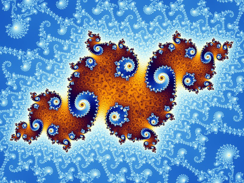
Answer: Fractals are like that; they are geometric figures that can be decomposed into smaller parts that are approximate and proportionally reduced copies of the whole. Recur-sions are like that again, or a little more convenient. Both (Practice), the functions in which the defining function is applied again within the definition are widely used in prog-ramming.
Peeling an onion is a vivid flow of recursion, with the last layer, when peeling is no longer possible, as the base layer. A family tree is a slightly better example, where for each parent we sea-rch for their parents (the children's grandparents), all the way down to those for whom we can no longer find an ancestor.
Without base cases, recursive calls can get out of control (stack overflow), and recursive solutions can be slower than others due to excessive memory usage. These two important recommendations are for computer scientists, but they also tell us something important about this information theory in general. I will only dwell on those that I have not emphasized before.
1. When a phenomenon is determined to be "real" (observable, permanent, and true), then what is unique is separated out, and what remains repeatable remains. Those parts that are not concrete are theoretical, repeated multiple times in many places and ways. In short, the "real" includes both concrete and abstract phenomena, the former being distinguished from the latter by diver-sity and redundancy.
Obviously, the fractals have repeatability as mentioned. However, when we find them in reality, we encounter their inconsistency. Thus, in the upper left image, the "island" represented by fractals can have a finite surface area but an infinite perimeter. Another example of a fractal pattern would create the law of large numbers by changing the macro in relation to the micro world. Similar to this is the change in the volume of a body with the cube of the length and the surface with the square.
2. Maze-solving programs often use recursion. We do not discuss their varia-nts here, but note that the inefficiency of such methods is not inherent in the nature of reality. It is not in the nature of the behavior of particle-waves, ma-terial particles, or larger bodies to learn all possible paths between two points of their movement in order to find the shortest distances, travel times, or the least expenditure of action. Such a waste of resources would contradict the requirements of general economy.
Instead of wasting memory, searching around, and time, there is basically minimal messing around, but one that is always consistent with itself. It turns out that nature can and does function that way. In the case of the inanimates, it is enough to adhere to the principle of least action blindly. This also happens with the presence of vitality, but it is less visible, and it is easier to say that than the principle of minimalism applies.
3. Preserving the past would have the same problem with efficiency if it were to adhere to ultimate consistency and determinism. Reality is such that it lasts and therefore has a growing past. The possibility of remembering the past, its constancy and truthfulness, makes it real, and in this theory, it is also inform-ative to its ongoing future (our present). Therefore, history is constantly fadi-ng, losing information about itself, and the older it is in this sense, the more likely it is to be thinner.
If the past were to change, in addition to radiating information towards the states of its origins (the present), it would overload reality and would not maintain its totality. What was (very much) a one-way flow of information, precisely because it is part of reality (which conserves the amount of inform-ation). For themselves, events from the past can also flow in other directions, as far as this theory is concerned, and can even be scattered everywhere until their flow to the present is (not) exactly sufficient for the law of conservation.
4. A change in an event that our present does not perceive, simply put, would be the development of that event in other dimensions of time. More precisely, this concerns this theory and is an acceptable explanation for it. Thus we come to the previously mentioned, and now inspired by fractals, priority of the stat-us quo as unifying over the principle of least action of theoretical physics and the principle of minimalism of this information theory.
Reality requires immutability, but it also allows for fiction. For example, just as we have the conservation of total energy along with the changing of its for-ms, or in mathematics, islands of pure truths connected by (Bridging) untru-ths, so we leave the possibility of reality residing even where we are not. An event (A) of our (B) past, when it is the past and some (C) parallel realities, according to the requirement of this theory, constitute a single community of realities (A-B-C). However, you can call the first (A) the pure reality, the second (B) the past, and (C) pseudo-reality.
In and Out » srb
Question: What is the internal and external information?

Answer: The question concerns non-trivial phenomena, first on “information of perception”, and second on “commutators” and further applied to central forces, especially Kepler's second law. It would therefore be too banal to talk about information that we store or do not store for something, or the like, so I will leave such parts of the answer for another occasion.
1. Let us pay attention to Maupertuis's principle of conservation of action (S = mvx). Nature tends to keep the product of mass, momentum and distance, or momentum and distance, constant. This is what I am talking about in the "inf-ormation of perception", here it is. Intelligence I, in the sense of the ability or power to process information, is directly proportional to action S, understood as a certain "quantity of possibilities", and inversely proportional to H, i.e. to the hierarchy, say to the constraints. Thus, I = S/H, and hence S = IH.
I understand this formula broadly, not only applied to physical matter but also to living beings. Thus, greater intelligence leads to greater activities, which is thus greater freedom, but greater such exertion will also be helped by an incr-ease in hierarchy. It is an unusually simple and very far-reaching formula abo-ut phenomena that are only partly intuitively easy to understand. For examp-le, the previous answer stated “the priority of the status quo as unifying over the principle of least action and the principle of minimalism.”.
2. Similar to Newton's (1687) bodies remaining in states of rest or uniform rectilinear motion unless acted upon by other bodies or forces, here we find the tendency of information (the quantity of options) to maintain the status quo, in addition to all previous physical matter. Just as a body that has som-ehow arrived at a state of, say, greater kinetic energy and seeks to maintain it, so too will an unlikely event, once it has occurred, seek to persist.
The causes are different from these similar effects. In a body that is in motion, some kinetic energy has been acquired, which it would have released at any convenient time, but which does not occur, as in an uncertain phenomenon, which is equal to the accumulation of some energy, impulse, then certainty that continues its duration. After all, for total uncertainty, or information, some conservation laws apply that will not allow their disappearance just like that.
3. By such a comparison, we arrive at internal and external information as proper velocity, as the object sees itself from its own frame, i.e. the system resting, measured by its own (proper) time, which flows slower than relative time, versus the external speed at which the body is seen by a relative obser-ver. Both have some "laws of inertia," each in a special way. The first infor-mation lies in the structure of the body, and the second is how the body communicates with its environment.
Observed in a single plane (Oxy), with only two degrees of freedom, x and y, the first and second information (depending on the definitions of the vectors, states A and B) are:
A⋅B = {A, B} = axbx + ayby = ab cos φ,
A×B = [A, B] = axby - bxay = ab sin φ,
where the angle φ = ∠(AOB) represents the displacement between the given states. Previously, I wrote these, the perceptual information and the commu-tator, as a scalar or vector product, using parentheses, i.e. the product of the intensity and the cosine and sine of the angles, and so it is here. It can also be written like this:
ab eiφ = ab(cos φ + i sin φ),
where i² = -1. This is the total information (of real quantities) written as a complex number.
4. When a body finds itself in front of a barrier of a large deficit or excess of external information, it will not easily cross it, just as it will generally not renounce the present or accept additional internal, coupled information. Little by little it will enter, say, the gravitational field into which the body enters, I believe, renouncing excess information, going towards places that are more likely to it. The opposite type of barrier is between parallel realities.
Parallel realities, if they existed as additional dimensions of time, would have the same bodies (in similar ways), therefore filled capacities, i.e., equal total amounts of information (energy), and would be repulsive to bodies on the other side. At the same time, when a case is realized with one outcome in one reality and with another in the other, those two outcomes become repulsive to each other and remain trapped in their environments.
5. External information (Conics) is related to the "forces" that act on parts of the body from the environment. In cases of points from which there are no such actions if such were the only ones, the body would move uniformly in a straight line, but such are rare or very distant. Therefore, the environment will almost certainly communicate (interact) with everybody, so it matters whether it is oversaturated as, say, in a parallel reality.
Barrier » srb
Question: Are you sure that "oversaturation" is the main cause of the separa-tion of "parallel realities"?
Answer: Of course not. Not only does such oversaturation seem to me to be the main cause of the se-paration of worlds, but it does not even seem to me to be an ordinary cause. However, if I am speculati-ng, I try to make it seem like I am predicting, but once something is established as absolutely certain, it becomes boring.
1. The probability of event A given that event B has occurred is the conditional probability, which we denote by Pr(A|B). Event A is independent of event B when Pr(A|B) = Pr(A), if the conditional probability and probability are equal. Also, events are independent if Pr(AB) = Pr(A)Pr(B), that is, when the proba-bility of their intersection (both together) is equal to the product of their pro-babilities. Moreover, if events A and B are independent, then they are not mu-tually exclusive (Independence).
On the other hand, if events A and B are mutually exclusive, then they are de-pendent. For example, the aforementioned “parallel realities” are not indepe-ndent because they have some common starting points in the realizations that led them to different outcomes. Such is the moment of the dilemma of falling “tails” or “heads” of a tossed coin when each of the outcomes goes to a differe-nt reality, or the freedom of our will to decide whether we want this or that by which we choose the future. This tells us that "parallel realities" are mutually exclusive.
2. A similar thing happens with the collapse of a superposition of a quantum state into one of the observables of a given measurement. Such observables are mutually exclusive because they emerged from the same superposition. They then lead their separate lives in “parallel realities” in the manner of en-tities that cannot communicate with each other. Such separations resemble the disintegration of a body and the separation of its particles, which then move away, never to meet again.
I personally like this reason for separating "parallel realities" more than the aforementioned oversaturation, but it doesn't cost me anything to try those alternatives. Note that this is still my private site, and its quotes are not for public publication. That's why they are interesting for me to research. I mean, if I know that parallel realities really exist, who knows if I would even deal with them?
3. Let's see what interesting alternative thinking could produce from the follo-wing example. Two objects moving away will see the redshift of the other (ph-otons). This means stretching out all the wavelengths of light, the original on-es they would have, or their increases in "position uncertainty" in the interpr-etation of Heisenberg's uncertainty relations. Consequently, they go towards greater certainty.
This parallel with the march towards greater certainty is particularly suited to the understanding of “all of the present” as a body moving away from uncerta-inty, that is, away from the past, since the body that is moving away is further and further into that past. The body that is approaching us has shortened wa-velengths of light, hence positions of smaller uncertainties, and on the other hand, according to special relativity, it comes to us from the future. With the former, we are more likely to move towards the future.
4. Now, on the other hand, we again come to the conclusion that the “parallel realities” are separated by the impossibility of communication (not anything communicates with anything), rather than the “oversaturation,” which is often also a barrier between (some). So, after considering both possibilities, at least we know that these two interpretations are real alternatives, that they are mu-tually exclusive, or that we can take one without the other. The open questions remain: how much is united in each of the “parallel realities,” what holds them together, and how to find related outcomes.
|
|
|