|
|
|


Here I am trying to answer the questions I received about the conservation la-ws, the Hamiltonian and the Lagrangian, the principle of least action, and ma-intaining the status quo in these situations. These are well-known points of th-eoretical physics, and they are so important because all its other laws are deri-ved from them. I will especially focus on information theory, including my own, where and how possible.
Mass IV » srb
Question: How to derive relativistic mass change?
Answer: Watch the video link to the image on the right that derives the expression for relativistic mass from collisions and conservation of momentum using Lorentz transfor-mations for velocity. I derived the same expression for mass in a dif-ferent way here (Mass III, 3), for calculating the energy dissipation (dE = F dx) with the work done by the force on the way. I will explain those two and list one more, the third way of performing a relativistic mass change.
1. In the video, the system S' moves away from the system S along the abscissa (x-axis) uniformly with a velocity v. In this system S', two bodies of equal mas-ses m' slide along the abscissa with uniform velocities u' and -u' until they col-lide when they stop. From the system S, these velocities u1 and u2 can be fou-nd from the Lorentz transformations, and the masses m1 and m2 are calculat-ed using the law of conservation of momentum:
$$ m_1\ u_1 + m_2\ u_2 = (m_1 + m_2)\ v $$ $$ m_1\ \frac{u'+v}{1 + \frac{u'v}{c^2}} + m_2\ \frac{-u'+v}{1 - \frac{u'v}{c^2}} = (m_1 + m_2)\ v $$ $$ m_1 \left(\frac{u'+v}{1 + \frac{u'v}{c^2}} - v\right) = m_2 \left(v - \frac{-u'+v}{1 - \frac{u'v}{c^2}}\right) $$ $$ \frac{m_1}{m_2} = \frac{1 + \frac{u'v}{c^2}}{1 - \frac{u'v}{c^2}} = \frac{1 + \eta}{1 - \eta}. $$We introduce a shorthand notation, η = u'v/c², for a more concise calculation:
$$ u_1^2 = \left(\frac{u'+v}{1 + \eta}\right)^2 = \frac{u'^2 + v^2 - c^2 - c^2\eta^2}{(1 + \eta)^2} $$ $$ u_2^2 = \left(\frac{u'+v}{1 + \eta}\right)^2 = \frac{u'^2 + v^2 - c^2 - c^2\eta^2}{(1 - \eta)^2} $$ $$ \frac{(1 + \eta)^2}{(1-\eta)^2} = \frac{u_2^2 - c^2}{u_1^2 - c^2} = \frac{1 - \frac{u_2^2}{c^2}}{1 - \frac{u_1^2}{c^2}} $$ $$ \frac{m_1}{m_2} = \frac{1 + \eta}{1 - \eta} = \frac{\sqrt{1 - \frac{u_2^2}{c^2}}}{\sqrt{1 - \frac{u_1^2}{c^2}}}. $$We choose the velocity v so that in the system S the second mass is at rest, tag by m0 = m2, so:
$$ m_1 = \frac{m_0}{\sqrt{1 - \frac{v^2}{c^2}}} $$because then u1 = v. The mass at rest m0 moving at speed v will be m1. This is the required relativistic increase in the mass of a body moving at speed v, wh-ere is c ≈ 300 000 km/s the speed of light in a vacuum.
2. We often write the same relativistic mass change, m = m0γ, where:
$$ \gamma = \frac{1}{\sqrt{1 - \frac{v^2}{c^2}}} $$is called the Lorentz parameter gamma. The Lorentz transformations give us both a length contraction Δℓ = Δℓ0/γ and a time dilation Δt = Δt 0γ, where Δℓ0 and Δt 0 are the units of length and time at rest. The similarity of these formu-las to relativistic mass is a consequence of the same. The slowing down of time for a moving system is compensated by its increase in mass. In this collision, the mass m is increased by just as much as the time is slowed down in order for the two masses to come to a complete stop in the system S'.
Namely, the work done by the force F on the path x is equal to the change in kinetic energy Ek, so:
$$ E_k = \int_{x_1}^{x_2} F\ dx = \int_{x_1}^{x_2} \frac{dp}{dt}\ dx = (m - m_0)c^2. $$The relativistic momentum p = mv is equivalent to Newton's second law with relativistic mass, whose change with time is force. The difference in masses in parentheses is the aforementioned mass increment, which is therefore kinetic energy and the relativistic formula for the equivalence of mass and energy, E = mc². Thus, the total energy of a body is the sum of this kinetic and rest energy:
E = (m - m0)c² + m0c² = mc².
This gives the upper integral in the aforementioned calculation (Mass III, 3), otherwise in which energy was the topic.
3. The same can be done a little differently. Force $\vec{F}$ is a vector quantity, mo-mentum $\vec{p} = m\vec{v}$ is a vector quantity, velocity $\vec{v}$ is also a vector quantity, and mass m is a scalar. So, since force is the change in momentum over time, we derive:
$$ \vec{F} = \frac{d(m\vec{v})}{dt} = m\frac{d\vec{v}}{dt} + \vec{v}\frac{dm}{dt}. $$There are vectors in the same direction, let's say abscissas, and the force on the path does work, and there it is energy in infinitesimal portions dE = Fdx, so we further have:
$$ dE = F\ dx = m\frac{dx}{dt}dv + v\frac{dx}{dt}dm = mv\ dv + v^2dm, $$ $$ dE = c^2dm = mv\ dv + v^2dm. $$The sequel is a matter of arrangement and integration:
$$ (c^2 - v^2)dm = mv\ dv $$ $$ \frac{dm}{m} = \frac{v}{c^2 - v^2}dv $$ $$ \int_{m_0}^m \frac{dm}{m} = \int_0^v \frac{v}{c^2 - v^2}dv $$ $$ \ln m \Bigg|_{m_0}^m = -\frac12\ln(c^2 - v^2)\Bigg|_0^v $$ $$ \frac{m}{m_0} = \sqrt{\frac{c^2}{c^2 - v^2}} $$ $$ m = \frac{m_0}{\sqrt{1 - \frac{v^2}{c^2}}}. $$That m is the same upper relativistic mass of a body moving at a velocity v, and whose rest mass is m0.
4. Information has the structure of packages. Particularly emphasized here are quanta, more precisely the products of energy changes over time (ΔE⋅Δt) whi-ch are of the order of Planck's constant. With the above expressions we can see them in the form of the product of force with position changes over time pass (F⋅Δx⋅Δt), especially due to the force of probability. The physics of information is about action, at least as far as this (my) theory of information is concerned. That is why we often have more probable outcomes, because they are less informative and transmit smaller actions, or vice versa. Faster movements create larger mass bases in additional dimensions of time, loss of events and slowing down of time, and this is also a tenacious (hypo)thesis of this theory.
Relativity II » srb
Question: What is the relationship between information theory and the theory of relativity?
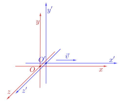
Answer: In the figure on the left, for example, there are two inertial frames Oxyz and O'x'y'z' whose coordinate axes coincide at the "initial" moment. When t = t' = 0, then x = x', y = y' and z = z', but the second frame moves with a uniform velocity v along the x-axis (abscis-sa), as in the answer above. This is the "right" Cartesian rectangular coordinate system; if the fingers of the right hand go in the direction x → y, from the abscissa to the ordi-nate, then the thumb points in the direction of the applicate (z-axis).
1. The first system moves with a velocity -v on the abscissa relative to the sec-ond. The principle of special relativity (Einstein, 1905) says something more, when these movements are uniform v = const. and in the absence of external forces, the laws of nature are equally valid in relation to each of the systems. In particular, the speed of light in a vacuum c = 299 792 458 m/s is the same in both. From these two Einstein principles (relativity and constant speed of light) the Lorentz transformations can be derived (Space-Time, p. 87):
$$ x'_0 = \gamma(x_0 - \beta x_1), \quad x'_1 = \gamma(x_1 - \beta x_0), \quad x'_2 = x_2, \quad x'_3 = x_3, $$ $$ \beta = \frac{v}{c}, \quad \gamma = (1 - \beta^2)^{1/2} = \frac{1}{\sqrt{1 - \frac{v^2}{c^2}}}. $$Here I have used the usual notations of the theory of relativity, x0 = ct, x1 = x, x2 = y and x3 = z. The time t has been replaced by the path x0 that light travels at a speed c during that time, thus avoiding differences in physical dimensions (second and meter), and the symmetry of the direction of motion and such "ti-me" is also noticeable. These transformations make Maxwell's equations inva-riant (Space-Time, p. 89), which is shown as a great confirmation of Einstein's principles of special relativity.
2. Lorentz transformations are not invariant in accelerated systems, especially in a gravitational field, and this problem troubled Einstein for about ten years until he came up with the equations of general relativity:
$$ R_{\mu\nu} - \frac12 R g_{\mu\nu} + \Lambda g_{\mu\nu} = \kappa T_{\mu\nu}, $$where the above coordinate indices are used, unless if only the time x0 = ct is replaced by the imaginary x4 = ict, which does not matter because it is squared everywhere in the development, and i² = -1. The new constant is κ = 8πG/c4 ≈ 2.07665×10-43 N-1, and G is the gravitational constant.
In a weak gravitational field, say Newtonian and no stronger than the solar system, the Schwarzschild metric holds:
$$ ds^2 = \left(1 - \frac{r_s}{r}\right)c^2dt^2 - \left(1 - \frac{r_s}{r}\right)^{-1}dr^2 - r^2d\Omega^2, $$ $$ d\Omega^2 = d\theta^2 + \sin^2\theta \ d\phi^2, \quad r_s = 2GM/c^2, $$in the spherical coordinate system $Or\theta\phi$, and M is the mass of the source body and rs is the Schwarzschild radius, or the radius within which the gravity of the black hole prevails. Einstein found the above system of equations (1916) by searching for invariants using tensor calculus, and developing Galileo's princi-ple of inertia into the equivalence principle.
Einstein's so-called strong equivalence principle states that the outcome of any local, non-gravitational test experiment is independent of the velocity of the experimental apparatus relative to the gravitational field and is independ-ent of where and when in the gravitational field the experiment is performed. "Local" means that the experimental setup should be small compared to the variations in the gravitational field. This is the "strong" equivalence principle, an extension of the previous one now called the "weak" equivalence principle, also known as the universality of free fall, or Galileo's principle.
3. If we talk about my information theory, then uncertainty is an objective ph-enomenon, it is unavoidable and must be visible in the foundations of all phy-sics, including the theory of relativity. However, it has not been there until now. According to the Chebyshev's inequality:
\[ \Pr[|X - \mu|\ge r] \le \frac{\sigma^2}{r^2}, \]probability decreases with the square of the distance. Here, when X are ran-dom variables of an arbitrary probability distribution, r is one of the values, where μ is the mean value, the so-called mathematical expectation, and σ² is the variance, or the mean square deviation from the mean value.
Such inequalities of large numbers in probability theory (there are more of them) instruct us on how to consider probability forces. Additionally, in the script Information Coupling (1.2.4 Conic Sections, and so on) I have listed theorems related to the topic, many of which are well-known, although not in this order, that all central constant forces decrease with the square of the dis-tance. Then, they push charges along conics (ellipses are attractive, hyperbolas are repulsive, and straight lines are zero). Gravity is such a non-zero attractive force, and special relativity speaks of zero forces.
4, Such a “probabilistic environment” has the status quo, when either-or cho-ices are equally likely. However, nature spontaneously avoids homogeneous distributions of chances, because they are the most informative. It tolerates them as if they were its basic fabric, without which it would not exist, or it sp-ontaneously finds a way out in stratification. There is no essential difference between uniform movements, except that for a long-term view (in billions of years) the universe is not symmetric in time. It constantly evolves from a less into more certain present, following the principle of minimalism.
Hyperspace » srb
Question: What do we get with imaginary time in these equations?
Answer: We are still discussing the relationship between information theory and relativity. The time no-tation x0 = ct translates time into length, and the notation x4 = ict, with an imaginary unit, i² = -1, in-troduces the calculus into hyper-space, which in mathematics and physics represents dimensions be-yond the range of direct observat-ion.
1. The first is the Minkowski space with 4-dim invariant length:
ds² = dx1² + dx2² + dx3² + dx4² = = dx² + dy² + dz² + (icdt)² = dℓ² - c²dt² = -c²(1 - v²/c²), ds² = -c²γ².
Hence this interval is an imaginary number, ds ∈ ℂ, because the speed of light and the Lorentz gamma are real. We avoid this with ds² = c²dt² - dℓ² = c²γ², but then some interesting things become obscured that we will discuss here. Both cases for this zero hyperdistance, ds = 0, provide a convenient compari-son for two systems, a body at rest in S and moving with velocity v relative to S'. We cancel the signs, and calculate:
ds² = ds'², c²dt² = c(1 - v²/c²)dt'², dt' = dt/(1 - v²/c²),
and that is the well-known formula for time dilation, where in S the clock is at rest, and from S' these durations are seen to be elongated.
2. Lorentz transformations become hyperbolic rotations in the plane Ox1x4 after the shift ct → ict, i.e. x0 → x4:
x' = γ(x - βct), ct' = γ(-βx + ct), x'1 = γ(x1 - βx4), x'4 = γ(-βx1 + x4), x'1 = cosh(φ) x1 - sinh(φ) x4, x'4 = -sinh(φ) x1 + cosh(φ) x4, cosh(φ) = γ, sinh(φ) = βγ, cosh²(φ) - sinh²(φ) = 1.
The hyperbolic cosine and hyperbolic sine functions were introduced, else:
$$ \cosh(\varphi) = \frac{e^\varphi + e^{-\varphi}}{2}, \quad \sinh(\varphi) = \frac{e^\varphi - e^{-\varphi}}{2}, $$which in the East are also denoted by ch(φ) and sh(φ). Now we can easily find:
eφ = γ(1 + β), e-φ = γ(1 - β),
so it is really eφ e-φ = 1. On the other hand, we have:
$$ \begin{pmatrix} x'_1 \\ x'_4 \end{pmatrix} \begin{pmatrix} \cosh \varphi & -\sinh \varphi \\ -\sinh \varphi & \cosh \varphi \end{pmatrix} \begin{pmatrix} x_1 \\ x_4 \end{pmatrix} $$rotation in hyperbolic space, x' = Rh(φ) x, for the "angle" φ. The determinant of that matrix, the hyper-rotation is also one, det(Rh) = 1. It is an isometry and therefore an expression of the law of conservation of motion.
In ordinary rotation (spatial coordinates), time t can be a factor of the angle and that rotation lasts and lasts, it is an isometry that conserves angular mo-mentum. In this, hyper-rotation, time x4 = ict is the coordinate that rotates and there is no conservation of duration, because that would be the conser-vation of spontaneous acceleration. These transformations do not change when we keep x0 instead of x4.
3. Uniform rectilinear motion is in conditions of equal probabilities, say equal wavelengths of bodies in motion, because such are traced by the uncertainty of their position. That is why Lorentz transformations are given by only one par-ameter, the velocity v, and perhaps also by the quotient beta (v/c). However, inertial motion through a gravitational field is in an environment of unequal probabilities that should be determined by at least two parameters. Let us choose a fall from rest outside the field into the central gravitational field, or zero initial velocity at infinity, more precisely v → 0 when r → ∞.
We use the Schwarzschild metric, so we can assume in advance the need for the coefficient γ = 1/(1 - rs/r) and the coefficient χ that depends on the velocity as well. This was a novelty when I stated it in the book Space-Time (2017) pp. 96-98, and now I will just retell it. The idea is to translate Lorentz transform-ations into local gravitational fields of a planet of mass M at a distance r from the center. In this spherical coordinate system $Or\theta\phi$ we can ignore the angles $\theta$ and $\phi$ which are then not transformed. Let's pay attention only to the radius $r$ and the time $t$. Starting from:
dr = αrrdr' + αrtcdt', cdt = αtrdr' + αttcdt',
by shifting to the Schwarzschild interval and looking for invariance, ds'² = ds², after squaring, adding and equating the coefficients we find the system of equ-ations:
$$ \begin{cases} dr = \chi\ dr' + i\gamma^{-1} \sqrt{1 - \gamma^2\chi^2}\ cdt' \\ cdt = i\gamma \sqrt{1 - \gamma^2\chi^2}\ dr' + \gamma^2\chi\ cdt' \end{cases} $$The details of the solution are in the aforementioned book, but by assuming them, it is easier to notice the analogy of the invariance of the Minkowski in-terval (which is a flat space-time) to Lorentz transformations and the invari-ance of the Schwarzschild interval to these transformations. The point is that these transformations are a direct translation of the Lorentz transformations into gravitational ones.
4. Transformations of gravity are isometry, but they are not rotations except for M = 0. This shows us that a material point in its infinitesimal gravitational environment is not under the influence of external forces. It is absurd, but in fact it is not, because in free fall the body is in a weightless state. This is a co-nfirmation of the above-mentioned principle of equivalence. Whether to take imaginary time (x4 = ict) or not (x0 = ct) in these calculations seems, at least for now, to be a matter of working method rather than final results.
Holonomy » srb
Question: Can you tell me in simple terms why and how space is curved by gravity?
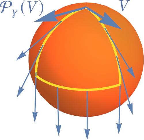
Answer: When we walk on a sphe-rical planet and always hold a spear in the same direction, it may happ-en that after traveling a full closed path, this spear will point in a diff-erent direction. We can see this in the image on the left, and the link explains holonomy.
The mathematical concept of holo-nomy describes the change in a ve-ctor that is translated along a clos-ed loop, returning to the starting point. It is a way of measuring the curvature of space by changing the orientation of an object after being moved. For example, two bodies in free fall at different locations on a planet may maintain their orientations relative to the line of descent (e.g. perpendic-ular to the radius) but these directions will change with respect to each other. Since bodies in free fall are weightless, as if free from forces, a change in said orientation will tell them that they are in curved space.
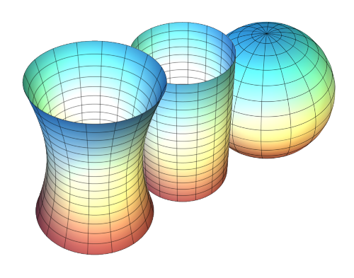
The link to the right explains curv-ed surfaces using the Gaussian me-thod (1827). When at a point on a surface we place two perpendicular circles of radius r1 and r2 that are (locally) tangent to it, it will be:
$$ K = \kappa_1\kappa_2 = \frac{1}{r_1}\frac{1}{r_2} $$that is the Gaussian curvature of the surface. In the figure, the first is hyperbolic and the second cylindri-cal, so the third is a spherical surface. The first has negative Gaussian curva-ture, because the signs of κ1 and κ2 are opposite (the circles are on different sides of the hyperboloid). The second has zero curvature due to the infinite radius of one of the circles. The third has positive curvature. This idea was developed by Riemann (1854) and applied to the curvature of space of arbit-rary dimensions. For example, a spherical surface cannot be represented on a flat map without deformation, because their curvatures are different, nor will inertial motion in a gravitational field be like rectilinear motion outside.
It is shown that the divergence of vectors in free fall, which smoothly follow geodesic lines while remaining parallel to themselves locally, means the same as holonomy, that they diverge globally and vice versa. Galileo's, Newton's and Einstein's physical concept of this is motion by inertia, i.e. the recently menti-oned equivalence principle (locally, there is no difference between upward ac-celeration and gravity). This is known in physics, but not the principle of mini-malism with which I am theorizing here and by which nature is self-regulati-ng. Avoiding uncertainty regarding the level of probabilities or their changes, by gradually adjusting them, can create an inertial motion that "fools" us into perceiving floating, whether as stationary or sliding "without external forces."
Manifold » srb
Question: After these contributions (Invariant III) I finally got the hang of co- and contra-variant vectors. Can you explain covariant differentiation to me in the same way?
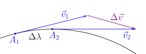
Answer: Let's imagine an infinite-simal situation like the one in the oversized drawing on the right. The vector $\vec{v} = \vec{v}(A)$ slides along the points (A) of the curve and when it travels the path Δλ from point A1 to point A2 changes by $\Delta\vec{v} \approx \vec{v}_2 - \vec{v}_1$, and this change is the vector by which the given vector tangents the given cur-ve at the given point A ∈ (A1, A2) of that very small interval (A1 ≈ A2). If vector $\vec{v}$ is not tangent, $\Delta\vec{v}$ will be. Second, the quantity $\Delta\vec{v}/\Delta \lambda$ is not infinitesimal, although the numerator and denominator are. Covariant differentiation will be to find the changes in the tangent vector $\Delta\vec{v}$ along the path $\Delta\lambda$.
1. This change is made by the partial derivative of the given vector with respect to lambda, also called the activity of the differentiation operator ∂/∂λ, or ∂λ:
$$ \frac{\partial \vec{v}}{\partial \lambda} = \frac{\partial}{\partial \lambda}\vec{v} = \partial_\lambda \vec{v}. $$In covariant differentiation, the paths of such lambdas are geodesics (the sh-ortest paths between given points, according to the metric of that space). We also represent them using vectors $\vec{e}_\mu$ of coordinate indices, say ct, r, θ, ϕ of a spherical system with, for example μ = 0, 1, 2, 3 if we have the space-time of the theory of relativity. In general, operators, including these $\partial/\partial \vec{e}_\mu$, simply ∂μ, form a vector space in which they are vectors. We write these operators:
$$ \vec{e}_\mu = \frac{\partial}{\partial x^\mu} = \partial_\mu $$and we treat them as covariant vectors.
2. The function s(x1, x2, ..., xn) of a given n-dim space has a differential:
$$ ds = \frac{\partial s}{\partial x^1}dx^1 + \frac{\partial s}{\partial x^2}dx^2 + ... + \frac{\partial s}{\partial x^n}dx^n, $$which, in this case, we can understand as the linear combination:
$$ d\vec{s} = \vec{e}_1dx^1 + \vec{e}_2dx^2 + ... + \vec{e}_ndx^n, $$ $$ d\vec{s} = \sum_{k=1}^n \vec{e}_k dx^k = \vec{e}_\mu dx^\mu. $$This final notation follows Einstein's convention of adding tensors by repeated subscripts and superscripts. We use tensors to describe invariant quantities, for example, relative motions in which physical laws apply equally. It is assu-med that the space in which the covariant differentiation is performed has an inner (scalar) multiplication, and then it has the intensity of the vector:
$$ \|ds\|^2 = \langle d\vec{s}| d\vec{s}\rangle = \sum_{j,k = 1}^n \langle \vec{e}_j | \vec{e}_k\rangle dx^j dx^k = g_{\mu\nu}dx^\mu dx^\nu. $$These values:
$$ g_{\mu\nu} = \langle \vec{e}_\mu | \vec{e}_\nu\rangle $$are called metric tensors and, as we can see, they define the intensity of a vector in our covariant differentiation space.
3. Example. Let us show that the small interval dℓ² = dx² + dy² + dz², i.e. the Pythagorean theorem 3-dim, in spherical coordinates (Orθϕ) is of the form:
dℓ² = dr² + r² dθ² + r² sin²θ dϕ²,
so, with non-zero metric coefficients:
grr = 1, gθθ = r², gϕϕ = r² sin²θ.
All other (mixed) metric coefficients are zero.
Instruction: We know the coordinate transformations:
$$ \begin{cases} x = r \sin\theta\cos\phi & x = x'^1 & r = x^1 \\ y = r\sin\theta \sin\phi & y = x'^2 & \theta = x^2 \\ z = r\cos\theta & z = x'^3 & \phi = x^3 \end{cases} $$then we calculate:
$$ g_{\mu\nu} = \frac{\partial x'^1}{\partial x^\mu}\frac{\partial x'^1}{\partial x^\nu} + \frac{\partial x'^2}{\partial x^\mu}\frac{\partial x'^2}{\partial x^\nu} + \frac{\partial x'^3}{\partial x^\mu}\frac{\partial x'^3}{\partial x^\nu} $$in order for all μ, ν ∈ {1, 2, 3}. However, these coordinates are orthogonal, which means that all the mixed scalar products are zero, ⟨r|θ⟩ = 0, ⟨r|ϕ⟩ = 0 and ⟨θ|φ⟩ = 0, together with the symmetry in the reverse order. It is always gμν = gνμ, and these mixed ones, μ ≠ ν, are zero in orthogonal systems. ∎
4. We have seen that the equivalence principle (Relativity II, 2) locally, within small regions of space-time, states that free fall is the same as floating in the space of an inertial frame. That is, that then the mass in gravity behaves the same as if it were in an accelerating rocket. In small space-times, we cannot establish the presence of gravity, i.e. we can always attribute the occurrence of gravity to some inertial or non-inertial frame, and we can eventually detect the presence of gravity in large regions of space-time.
This is consistent with the "accident" of the graviton (Graviton II, 4) that it has a spin 2 that cannot interact with small spin 1/2 fermions. It also agrees with the probabilistic explanation of gravity and the principle of minimalism. Thus, special relativity is locally indistinguishable from general relativity, and so an extension of the Lorentz transformations (Hyperspace, 3) makes sense. These are properties of the so-called "manifold", a curved space that behaves flat in a small local region. For example, the surface of the Earth is such a manifold and globally it is curved.
Geodesic » srb
Question: You said (Manifold), covariant differentiation gives the change in tangent vector $\Delta\vec{v}$ on the path $\Delta\lambda$, but you didn't provide the formula?
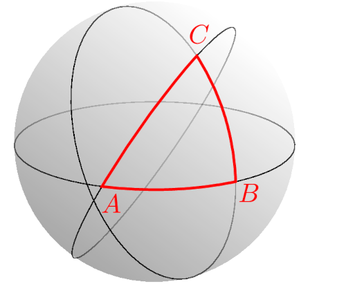
Answer: Yes, this formula requires more knowledge, but I will try to explain it as simply as possible. Fi-rst, we will understand the geodesic line, that it is the shortest line bet-ween two points, all inside a curved surface. Its special case is the “str-aight line” of flat space (Euclidean). Another example is the arcs, like AB, BC or CA in the image on the left, of the greatest circles of the sphere. They will be imitated by a string stretched between pairs of its points. Roughly, the surface of the earth is like this and we can take it as an example in the following understand-ing.
1. When we turn left or right in a car, changing the direction of speed, (cent-rifugal) acceleration appears and the movement is not along a geodesic line. But, when we overcome a hill or pass a depression and take the shortest route, the acceleration is perpendicular to the surface, first downward and second upward, which is movement along a geodesic line. So, by looking for these geodesics, we are looking for accelerations perpendicular to the surface.
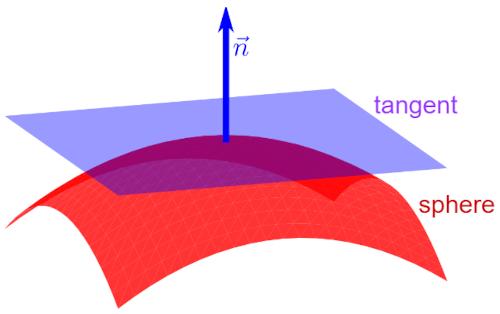
In the image on the right we see the red surface of the sphere, then the tangent plane and $\vec{n}$ the normal ve-ctor over both the sphere and the tangent. So, the accelerations a = d²f/dλ², the second derivatives of the function f(ξ, η) of the moveme-nt of the sphere along some of its coordinates ξ and η, along the re-quired geodesic λ should be sepa-rated into components, a = an + at, where the latter is zero, at = 0. The function f = f(x, y, z), where each of these coordinates depend on the coordinates ξ and η. These can be spherical coor-dinates with which we describe Cartesian ones, but they do not have to be. In the previous answer (3rd example) it would be r = 1, θ = ξ and ϕ = η. Further we work with such vector position functions $\vec{s} = \vec{s}(x,y,z)$.
2. For motion along a geodesic line only one degree of freedom is needed, then ξ = ξ(λ) and η = ξ(λ), so x = x(λ), y = y(λ) and z = z(λ). The unit vectors of tang-ential motion, the base velocities are:
$$ \vec{e}_\xi = \frac{\partial \vec{s}}{\partial \xi}, \quad \vec{e}_\eta = \frac{\partial \vec{s}}{\partial \eta}, \quad \vec{e}_\eta = \frac{\partial \vec{s}}{\partial \lambda} $$This third one is along the required geodesic line, a linear combination of the two basis vectors. This third velocity and acceleration are:
$$ \frac{d\vec{s}}{d\lambda} = \frac{d\xi}{d\lambda}\frac{\partial \vec{s}}{\partial\xi} + \frac{d\eta}{d\lambda}\frac{\partial \vec{s}}{\partial\eta}, $$ $$ \frac{d}{d\lambda}\left(\frac{d\vec{s}}{d\lambda}\right) = \frac{d}{d\lambda}\left(\frac{d\xi}{d\lambda}\frac{\partial \vec{s}}{\partial \xi}\right) + \frac{d}{d\lambda}\left(\frac{d\eta}{d\lambda}\frac{\partial \vec{s}}{\partial \eta}\right) = $$ $$ = \frac{d^2\xi}{d\lambda^2}\frac{\partial \vec{s}}{\partial \xi} + \frac{d\xi}{d\lambda}\left(\frac{d}{d\lambda}\frac{\partial \vec{s}}{\partial \xi}\right) + \frac{d^2\eta}{d\lambda^2}\frac{\partial \vec{s}}{\partial \eta} + \frac{d\eta}{d\lambda}\left(\frac{d}{d\lambda}\frac{\partial \vec{s}}{\partial \eta}\right). $$3. Let us further apply the well-known rule of differentiation:
$$ \frac{d}{d\lambda} = \frac{d\xi}{d\lambda}\frac{\partial}{\partial \xi} + \frac{d\eta}{d\lambda}\frac{\partial}{\partial \eta} $$twice, so we get:
$$ \frac{d}{d\lambda}\frac{\partial \vec{s}}{\partial \xi} = \frac{d \xi}{d\lambda}\frac{\partial^2 \vec{s}}{\partial \xi^2} + \frac{d\eta}{d\lambda}\frac{\partial^2 \vec{s}}{\partial \xi \partial \eta}, $$ $$ \frac{d}{d\lambda}\frac{\partial \vec{s}}{\partial \eta} = \frac{d\xi}{d\lambda}\frac{\partial^2 \vec{s}}{\partial \eta \partial \xi} + \frac{d \eta}{d\lambda}\frac{\partial^2 \vec{s}}{\partial \eta^2}. $$Plugging this into the previous acceleration, we find:
$$ \frac{d^2\vec{s}}{d\lambda^2} = \frac{d^2\xi}{d\lambda^2}\frac{\partial \vec{s}}{\partial\xi} + \frac{d^2\eta}{d\lambda^2}\frac{\partial \vec{s}}{\partial\eta} + $$ $$ + \left(\frac{d\xi}{d\lambda}\right)^2\frac{\partial^2\vec{s}}{\partial\xi^2} + \frac{d\xi}{d\lambda}\frac{d\eta}{d\lambda}\frac{\partial^2\vec{s}}{\partial\xi \partial\eta} + \frac{d\eta}{d\lambda}\frac{d\xi}{d\lambda}\frac{\partial^2\vec{s}}{\partial\eta \partial\xi} + \left(\frac{d\eta}{d\lambda}\right)^2\frac{\partial^2\vec{s}}{\partial\eta^2}. $$The first two sums are tangent vectors, and we don't know about the other four.
4. This, the notations ζ1 = ξ and ζ2 = η and the Einstein convention simplify:
$$ \frac{d^2\vec{s}}{d\lambda^2} = \frac{d^2\zeta^\mu}{d\lambda^2}\frac{d\vec{s}}{d\zeta^\mu} + \frac{d\zeta^\mu}{d\lambda}\frac{d\zeta^\nu}{d\lambda}\frac{\partial^2\vec{s}}{\partial\zeta^\mu \partial\zeta^\nu} $$where it is summed over repeated indices μ, ν ∈ {1, 2}. The first term is the sum of tangent vectors, we do not know the second, so let's consider its third factor. We write it in the form:
$$ \frac{\partial^2\vec{s}}{\partial\zeta^\mu \partial\zeta^\nu} = \Gamma^1_{\mu\nu}\frac{\partial \vec{s}}{\partial \zeta^1} + \Gamma^2_{\mu\nu}\frac{\partial \vec{s}}{\partial \zeta^2} + \text{II}_{\mu\nu}\vec{n}. $$The first two terms contain the yet-to-be-defined Christoffel symbols that give the tangential components of the expression in front of the equality, and the third is the Second fundamental form that gives the normal components. The first term gives the components of the first tangent vector (∂s/∂ζ1), the second term gives the second (∂s/∂ζ2), and the IIμν gives the perpendicular compone-nts. We write this more concise:
$$ \frac{\partial^2\vec{s}}{\partial\zeta^\mu \partial\zeta^\nu} = \Gamma^\alpha_{\mu\nu}\frac{\partial \vec{s}}{\partial \zeta^\alpha} + \text{II}_{\mu\nu}\vec{n} $$using Einstein's conventions.
5. The normal vector and the tangent are perpendicular by definition. This means that their scalar product is zero, $\vec{n}\cdot(\partial\vec{s}/\partial \zeta^\beta) = 0$, so we use this to separate the Christoffel symbols from the Second Fundamental Form:
$$ \frac{\partial^2\vec{s}}{\partial\zeta^\mu \partial\zeta^\nu}\cdot \frac{\partial \vec{s}}{\partial \zeta^\beta} = \left(\Gamma^\alpha_{\mu\nu}\frac{\partial \vec{s}}{\partial \zeta^\alpha} + \text{II}_{\mu\nu}\vec{n}\right)\cdot \frac{\partial \vec{s}}{\partial \zeta^\beta}, $$ $$ \frac{\partial^2\vec{s}}{\partial\zeta^\mu \partial\zeta^\nu}\cdot \frac{\partial \vec{s}}{\partial \zeta^\beta} = \Gamma^\alpha_{\mu\nu}\frac{\partial \vec{s}}{\partial \zeta^\alpha} \cdot \frac{\partial \vec{s}}{\partial \zeta^\beta}, $$ $$ \frac{\partial^2\vec{s}}{\partial\zeta^\mu \partial\zeta^\nu}\cdot \frac{\partial \vec{s}}{\partial \zeta^\beta} = \Gamma^\alpha_{\mu\nu}g_{\alpha\beta} $$because $(\partial_\alpha \vec{s})\cdot (\partial_\beta \vec{s}) = g_{\alpha\beta}$, i.e. the scalar product of tangent vectors is a metric tensor. Such a tensor multiplied by the inverse metric tensor (with the upper indices) cancels out, gαβ gβγ = δαγ, so:
$$ \Gamma^\gamma_{\mu\nu} = \frac{\partial^2\vec{s}}{\partial\zeta^\mu \partial\zeta^\nu}\cdot \frac{\partial \vec{s}}{\partial \zeta^\beta} g^{\beta\gamma}. $$Thus, we have determined the so-called Christoffel symbols $\Gamma^\gamma_{\mu\nu}$.
On the other hand, multiplying the previous equality scalarly by the normal unit vector, $\vec{n}\cdot\vec{n} = 1$, gives:
$$ \frac{\partial^2 \vec{s}}{\partial \zeta^\mu \partial \zeta^\nu}\cdot \vec{n} = \left(\Gamma^\alpha_{\mu\nu}\frac{\partial \vec{s}}{\partial \zeta^\alpha} + \text{II}_{\mu\nu}\vec{n}\right) \cdot \vec{n}, $$ $$ \frac{\partial^2 \vec{s}}{\partial \zeta^\mu \partial \zeta^\nu}\cdot \vec{n} = \text{II}_{\mu\nu}(\vec{n}\cdot \vec{n}), $$ $$ \text{II}_{\mu\nu} = \frac{\partial^2 \vec{s}}{\partial \zeta^\mu \partial \zeta^\nu}\cdot \vec{n} = \frac{\partial^2 \vec{s}}{\partial \zeta^\mu \partial \zeta^\nu}\cdot \frac{\vec{e}_\mu\times\vec{e}_\nu}{\|\vec{e}_\mu\times\vec{e}_\nu\|}. $$In the vector (external, cross) product, the tangent vectors are:
$$ \vec{e}_\mu = \frac{\partial \vec{s}}{\partial \zeta^\mu}, \quad \vec{e}_\nu = \frac{\partial \vec{s}}{\partial \zeta^\nu}. $$Thus, we have determined the so-called Second Fundamental Form IIμν.
6. To find the differential equations of motion, let's start with the acceleration (4) and in the second term (right), replace the third factor with a "more conci-se" one:
$$ \frac{d^2\vec{s}}{d\lambda^2} = \frac{d^2\zeta^\mu}{d\lambda^2}\frac{d\vec{s}}{d\zeta^\mu} + \frac{d\zeta^\mu}{d\lambda}\frac{d\zeta^\nu}{d\lambda}\left(\Gamma^\alpha_{\mu\nu}\frac{\partial \vec{s}}{\partial \zeta^\alpha} + \text{II}_{\mu\nu}\vec{n}\right), $$ $$ \frac{d^2\vec{s}}{d\lambda^2} = \left(\frac{d^2\zeta^\alpha}{d\lambda^2} + \Gamma_{\mu\nu}^\alpha \frac{d\zeta^\mu}{d\lambda}\frac{d\zeta^\nu}{d\lambda}\right)\frac{\partial \vec{s}}{\partial \zeta^\alpha} + \text{II}_{\mu\nu}\frac{d\zeta^\mu}{d\lambda}\frac{d\zeta^\nu}{d\lambda}\vec{n}. $$Geodesic curves are on paths where the acceleration vector is perpendicular to the surface. This means that (1) from the acceleration $\vec{a} = \vec{a}_t + \vec{a}_n$, which we also have in the formula just derived. The first part is the tangential accelera-tion, and the second term is the normal (orthogonal), and they are mutually perpendicular vectors:
$$ \vec{a}_t = \left(\frac{d^2\zeta^\alpha}{d\lambda^2} + \Gamma_{\mu\nu}^\alpha \frac{d\zeta^\mu}{d\lambda}\frac{d\zeta^\nu}{d\lambda}\right)\frac{\partial \vec{s}}{\partial \zeta^\alpha}, \quad \vec{a}_n = \text{II}_{\mu\nu}\frac{d\zeta^\mu}{d\lambda}\frac{d\zeta^\nu}{d\lambda}\vec{n}. $$Geodesic lines are those on which there is no tangential acceleration, so are:
$$ \frac{d^2\zeta^\alpha}{d\lambda^2} + \Gamma_{\mu\nu}^\alpha \frac{d\zeta^\mu}{d\lambda}\frac{d\zeta^\nu}{d\lambda} = 0 $$the required differential equations of geodesic lines. By solving them, we find geodesics, the so-called straightest possible paths of a curved surface, space.
Flat » srb
Question: Wow! I'm surprised by all the differentiation (Geodesic). Is there anything simpler?
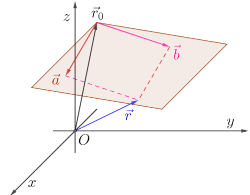
Answer: Tensor calculus is not in the program of amateurs in math-ematics, but you can start by calc-ulating geodesic lines of Euclidean planes, by checking equations (6). What would be the position vector $\vec{s}$ there, is seen in the figure on the left as a radius vector:
$$ \vec{r} = \vec{r}_0 + \xi\, \vec{a} + \eta\, \vec{b}, $$where $\vec{r}_0$, $\vec{a}$ and $\vec{b}$ are some const-ant vectors that define the (brown-hatched) plane whose points are indicated by the vector $\vec{r}(\xi, \eta)$. By changing ξ, η ∈ ℝ, arbitrary variables, all points of that plane are obtained. As is known, geodesics of the Euclidean plane are lines and here is how this is determined by solving the aforementioned differential equations.
1. So, on the given plane we test the differential equation of the geodesic:
$$ \frac{d^2\zeta^\alpha}{d\lambda^2} + \Gamma_{\mu\nu}^\alpha \frac{d\zeta^\mu}{d\lambda}\frac{d\zeta^\nu}{d\lambda} = 0, $$where the variables ζ1 = ξ and ζ2 = η, and all three vectors of the equation of the points of the given plane $\vec{r}(\xi, \eta) = \vec{r}_0 + \xi\, \vec{a} + \eta\, \vec{b}$ are constant. This is the position vector.
2. The first and second derivatives of the position vector are the velocity, and then the acceleration:
$$ \vec{e}_\xi = \frac{\partial \vec{r}}{\partial \xi} = \vec{a}, \quad \vec{e}_\eta = \frac{\partial \vec{r}}{\partial \eta} = \vec{b}, $$ $$ \frac{\partial^2 \vec{r}}{\partial \xi^2} = \frac{\partial^2 \vec{r}}{\partial \xi \partial \eta} = \frac{\partial^2 \vec{r}}{\partial \eta \partial \xi} = \frac{\partial^2 \vec{r}}{\partial \eta^2} = 0. $$The velocities are constant, and there is no acceleration. It is said that a curved surface has vertical accelerations, and this one has none at all, which means that it is not curved anywhere. Of course, this was expected and has now been confirmed.
3. Above (Geodesic, 5) general formulas for Christoffel symbols were found, which are now all zeros, because the first factor is the accelerations which are all zeros:
$$ \Gamma^\gamma_{\mu\nu} = \frac{\partial^2\vec{r}}{\partial\zeta^\mu \partial\zeta^\nu}\cdot \frac{\partial \vec{r}}{\partial \zeta^\beta} g^{\beta\gamma} = 0. $$From the above (1) differential equation of the geodesic, only the first term remains:
$$ \frac{d^2\xi}{d\lambda^2} = 0, \quad \frac{d^2\eta}{d\lambda^2} = 0, $$ $$ \frac{d\xi}{d\lambda} = a_1, \quad \frac{d\eta}{d\lambda} = b_1, $$ $$ \xi = a_1 + a_2\lambda, \quad \eta = b_1 + b_2\eta, $$where aj, bk ∈ ℝ are arbitrary constants. And these are parametric equations of straight lines, parameters λ ∈ ℝ.
4. We multiply the first by b2 and the second by a2 and subtract them — to eliminate the parameter λ. We get:
$$ b_2\, \xi - a_2\, \eta = a_1b_2 - a_2b_1, $$and these are equations of lines, depending on the constants aj and bk. Note that in this case, searching for geodesic lines of the Euclidean plane, we did not even have to calculate the metric tensor gμν.
5. This uncurved space of Euclidean geometry exists locally and perhaps quite globally to the limits of the visible universe. In between, in the range of sizes, there are galaxies, stars and planets, which make physical space-time curved. Let us note the analogy of these spatial sizes with the durations, the extensions of processes, which analogously have their local divergences and global conve-rgences. It would be difficult to understand such similarities, other than an optional theoretical phenomenon, if it were not for the principle of minimali-sm and its derivative that nature does not like equalities. I only mention it, as before, to remind ourselves of the scope of this principle.
Sphere II » srb
Question: Can you solve those equations (Geodesic, 5) for a sphere as well?
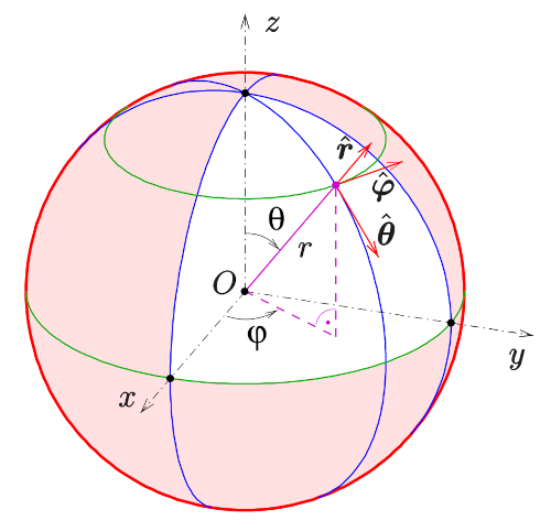
Answer: Spheres are everywhere in tensor calculus textbooks and are a bit of a hackneyed topic for this bl-og, but I agree for the sake of the observation that the degeneracy of flat space only occurs if perpendic-ular "forces" act on the surface. Th-is as a model of internal informati-on, but also as an analogy to virtual Spheres which are also outside of school routines. The story of indis-tinguishable particles is also an an-alogy to this, in the ways that we lo-cally do not distinguish accelerati-on from gravity (Manifold, 4).
1. We use our notations ζ1 = θ, ζ2 = φ and r = 1 for the usual parametric formu-las of spherical positions, from which we will find the velocities and accelerati-ons:
$$ x = \sin\zeta^1\cos\zeta^2, \quad y = \sin\zeta^1\sin\zeta^2, \quad z = \cos\zeta^1, $$ $$ \frac{\partial \vec{s}}{\partial \zeta^1} = \frac{\partial \vec{s}}{\partial x}\frac{\partial x}{\partial \zeta^1} + \frac{\partial \vec{s}}{\partial y}\frac{\partial y}{\partial \zeta^1} + \frac{\partial \vec{s}}{\partial z}\frac{\partial z}{\partial \zeta^1} = \vec{e}_1, $$ $$ \frac{\partial \vec{s}}{\partial \zeta^2} = \frac{\partial \vec{s}}{\partial x}\frac{\partial x}{\partial \zeta^2} + \frac{\partial \vec{s}}{\partial y}\frac{\partial y}{\partial \zeta^2} + \frac{\partial \vec{s}}{\partial z}\frac{\partial z}{\partial \zeta^2} = \vec{e}_2, $$where the position vector $\vec{s} = (x, y, z)$ is a point on a sphere of radius one with the basis velocity vectors $\vec{e}_1$ in the direction of the equator and $\vec{e}_2$ in the direction from the north to the south pole. We obtain:
$$ \vec{e}_1 = \frac{\partial \vec{s}}{\partial \zeta^1} = \frac{\partial \vec{s}}{\partial x}\cos\zeta^1\cos\zeta^2 + \frac{\partial \vec{s}}{\partial y}\cos\zeta^1\sin\zeta^2 - \frac{\partial \vec{s}}{\partial z}\sin\zeta^1, $$ $$ \vec{e}_2 = \frac{\partial \vec{s}}{\partial \zeta^2} = -\frac{\partial \vec{s}}{\partial x}\sin\zeta^1\sin\zeta^2 + \frac{\partial \vec{s}}{\partial y}\sin\zeta^1\cos\zeta^2 + \frac{\partial \vec{s}}{\partial z}\cdot 0. $$Let's calculate metric tensors in the meantime, $g_{\mu\nu} = \langle \vec{e}_\mu, \vec{e}_\nu\rangle$.
2. We find the metric tensor by scalar multiplication of the velocity vectors:
$$ g_{\mu\nu} = \vec{e}_\mu \cdot \vec{e}_\nu = \langle \vec{e}_\mu | \vec{e}_\nu\rangle = \langle \vec{e}_\mu , \vec{e}_\nu\rangle. $$Let's calculate the first of the four components μ, ν ∈ {1, 2}:
$$ g_{11} = \begin{pmatrix} \cos\zeta^1\cos\zeta^2 & \cos\zeta^1\sin\zeta^2 & -\sin\zeta^1 \end{pmatrix} \begin{pmatrix} \cos\zeta^1\cos\zeta^2 \\ \cos\zeta^1\sin\zeta^2 \\ -\sin\zeta^1 \end{pmatrix} $$ $$ = \cos^2\zeta^1\cos^2\zeta^2 + \cos^2\zeta^1\sin^2\zeta^2 + \sin^2\zeta^1 $$ $$ = \cos^2\zeta^1(\cos^2\zeta^2 + \sin^2\zeta^2) + \sin^2\zeta^1 $$ $$ = \cos^2\zeta^1 + \sin^2\zeta^1, $$ $$ g_{11} = 1. $$Similarly, we find g12 = g21 = 0 and g22 = (sin ζ1)². Therefore, the metric tensor gμν and its inverse gμν are, in summary:
$$ g_{\mu\nu} = \begin{pmatrix} 1 & 0 \\ 0 & (\sin\zeta^1)^2 \end{pmatrix}, \quad g^{\mu\nu} = \begin{pmatrix} 1 & 0 \\ 0 & (\sin\zeta^1)^{-2} \end{pmatrix}. $$As we know from earlier dΩ² = dθ² + (sin φ)²dφ², and we have that here too, i.e. the square of the interval on the sphere ds² = (dζ1)² + (sin ζ1)²(dζ2)².
3. The derivatives of velocity are accelerations:
$$ \frac{\partial^2 \vec{s}}{\partial (\zeta^1)^2} = -\frac{\partial \vec{s}}{\partial x}\sin\zeta^1\cos\zeta^2 - \frac{\partial \vec{s}}{\partial y}\sin\zeta^1\sin\zeta^2 - \frac{\partial \vec{s}}{\partial z}\cos\zeta^1, $$ $$ \frac{\partial^2 \vec{s}}{\partial (\zeta^2)^2} = -\frac{\partial \vec{s}}{\partial x}\sin\zeta^1\cos\zeta^2 - \frac{\partial \vec{s}}{\partial y}\sin\zeta^1\sin\zeta^2, $$ $$ \frac{\partial^2 \vec{s}}{\partial\zeta^1 \partial\zeta^2} = \frac{\partial^2 \vec{s}}{\partial \zeta^2 \partial \zeta^1} = -\frac{\partial \vec{s}}{\partial x}\cos\zeta^1\sin\zeta^2 + \frac{\partial \vec{s}}{\partial y}\cos\zeta^1\cos\zeta^2. $$Now we have all the vectors for scalar products, the Christoffel symbols:
$$ \Gamma_{\mu\nu}^\alpha = \frac{\partial^2\vec{s}}{\partial \zeta^\mu \partial \zeta^\nu} \cdot \frac{\partial \vec{s}}{\partial \zeta^\beta} g^{\beta\alpha}. $$We add up and down the same index (β = 1, 2), in two cases (α = 1, 2):
$$ \Gamma_{\mu\nu}^1 = \frac{\partial^2 \vec{s}}{\partial \zeta^\mu \partial \zeta^\nu} \cdot \frac{\partial \vec{s}}{\partial \zeta^1}g^{11} + \frac{\partial^2 \vec{s}}{\partial \zeta^\mu \partial \zeta^\nu} \cdot \frac{\partial \vec{s}}{\partial \zeta^2}g^{21}, $$ $$ \Gamma_{\mu\nu}^2 = \frac{\partial^2 \vec{s}}{\partial \zeta^\mu \partial \zeta^\nu} \cdot \frac{\partial \vec{s}}{\partial \zeta^1}g^{12} + \frac{\partial^2 \vec{s}}{\partial \zeta^\mu \partial \zeta^\nu} \cdot \frac{\partial \vec{s}}{\partial \zeta^2}g^{22}. $$The mixed coefficients of the metric tensor are zero, g12 = g21 = 0, so:
$$ \Gamma_{\mu\nu}^1 = \frac{\partial^2 \vec{s}}{\partial \zeta^\mu \partial \zeta^\nu} \cdot \frac{\partial \vec{s}}{\partial \zeta^1}, \quad \Gamma_{\mu\nu}^2 = \frac{\partial^2 \vec{s}}{\partial \zeta^\mu \partial \zeta^\nu} \cdot \frac{\partial \vec{s}}{\partial \zeta^2}\frac{1}{(\sin \zeta^1)^2}, $$because g11 = 1 and g22 = 1/(sin ζ1)². Then we calculate the scalar products, of which only the following two are non-zero:
$$ \frac{\partial^2 \vec{s}}{\partial (\zeta^1)^2} \cdot \frac{\partial \vec{s}}{\partial \zeta^1} = -\cos\zeta^1 \sin\zeta^1, \quad \frac{\partial^2 \vec{s}}{\partial \zeta^1 \partial \zeta^2} \cdot \frac{\partial \vec{s}}{\partial \zeta^2} = \cos\zeta^1 \sin\zeta^1. $$Note the symmetry of the lower indices, $\Gamma_{\mu\nu}^\alpha = \Gamma_{\nu\mu}^\alpha$, and we find:
$$ \Gamma_{22}^1 = -\cos\zeta^1\sin\zeta^1, \quad \Gamma_{12}^2 = \Gamma_{21}^2 = \frac{\cos\zeta^1}{\sin\zeta^1}, $$which are the only nonzero Christoffel symbols of the sphere.
4. We have all the elements of the differential equations of the geodesic lines of the sphere. Only two of the eight (2×2×2) remain:
$$ \frac{d^2\zeta^1}{d\lambda^2} + \Gamma_{22}^1\frac{d\zeta^2}{d\lambda}\frac{d\zeta^2}{d\lambda} = 0, $$ $$ \frac{d^2\zeta^2}{d\lambda^2} + 2\Gamma_{12}^2\frac{d\zeta^1}{d\lambda}\frac{d\zeta^2}{d\lambda} = 0, $$and when we include gammas, these are differential equations:
$$ \frac{d^2\zeta^1}{d\lambda^2} - \cos\zeta^1\sin\zeta^1\frac{d\zeta^2}{d\lambda}\frac{d\zeta^2}{d\lambda} = 0, $$ $$ \frac{d^2\zeta^2}{d\lambda^2} + 2\cot\zeta^1 \frac{d\zeta^1}{d\lambda}\frac{d\zeta^2}{d\lambda} = 0. $$As a reminder, these labels usually have the names ζ1 = θ and ζ2 = φ, and now we are working with a sphere of radius r = 1. This is easily generalized, as are the solutions that we do not calculate (it is unnecessarily extensive) but only check.
5. The angle ζ1 = θ is like latitude (it is is 0° at the equator), but as a deviation from north to south and let it be a constant, θ = θ0. The angle ζ2 = φ. It is oth-erwise the longitude that measures the east-west position, and let it be variab-le. Then φ = kλ. We easily find the first and second derivatives:
$$ \frac{d\theta}{d\lambda} = 0, \quad \frac{d\varphi}{d\lambda} = k, $$ $$ \frac{d^2\theta}{d\lambda^2} = 0, \quad \frac{d^2\varphi}{d\lambda^2} = 0. $$We insert them into the above differential equations and obtain:
$$ -\cos \theta_0 \sin \theta_0\, k^2 = 0, \quad 2\text{ctg}\, \theta_0 \cdot 0\cdot k = 0. $$The latter is the identity (0 = 0), and the solutions of the former are sin θ0 = 0 and cos θ0 = 0. These are θ0 = 0 and θ0 = 90°. The former gives only one poi-nt (the north pole), the latter is the equator (of various values of φ). The angl-es 0° < θ0 < 90° are not considered. This gives only the greatest circle of the sphere as a solution, and then symmetrically to this we have the other solutio-ns, all the greatest circles — intersections of the sphere and the plane passing through its center.
Gravity IV » srb
Question: Is it true that one can calculate the Schwarzschild interval and metr-ic tensor of the Einstein field from Newtonian gravity?
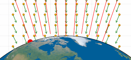
Answer: Yes, I've written about it so many times, even in the book Space-Time (p. 58), maybe even before, but it's not interesting en-ough to be accepted. Anyway, I'll repeat the part that concerns pre-vious geodesics so that, hopefully, it turns out a bit novel, and certa-inly in a different way than the previous blog (Gravity III).
We observe the vertical fall of a body of mass m from an initial rest at infinity towards a celestial body of significantly greater mass M. Gravity pulls down with Newton's force with the gravitational constant G:
$$ F = G\frac{Mm}{r^2}. $$The first example uses Newton's second law F = ma, to paraphrase, force on mass gives acceleration.
1. Example. Show that the velocity v = v(r) of a smaller body of mass m falling vertically from rest into the gravitational field of a body of mass M would be:
$$ v^2 = -2G\frac{M}{r}, $$at a distance r from the center of gravity, from the center of mass M.
Solution: The following equalities apply to forces, accelerations, and velocities:
$$ ma = G\frac{Mm}{r^2}, $$ $$ \frac{dv}{dt} = G\frac{M}{r^2}, $$ $$ \frac{dv}{dr}\frac{dr}{dt} = G\frac{M}{r^2}, $$ $$ \int_0^v v\, dv = \int_\infty^r G\frac{M}{r^2}\, dr, $$so after integrating, on the left from rest to the required speed v, and on the right from infinity to the height r, we find:
$$ v^2 = -2G\frac{M}{r} $$and that's what was supposed to be shown. ∎
2. Let's add a few insights from the special theory of relativity (Einstein, 1905), and without the general theory (Einstein, 1916). First of all, it is the dilation of time and the contraction of lengths along the direction of motion, which are relatively:
$$ \Delta t = \frac{\Delta t_0}{\sqrt{1 - \frac{v^2}{c^2}}}, \quad \Delta r = \Delta r_0 \sqrt{1 - \frac{v^2}{c^2}}, $$where Δt0 and Δr0 are the proper time and length, i.e. of the body at rest. Wh-en a body falls inertially in a gravitational field, we now say, it passes through the relative times (t) and radial (r) lengths of those positions, while the perpe-ndicular coordinates (θ and φ) will remain unchanged. Hence the interval:
$$ ds^2 = \left(1 - \frac{2GM}{rc^2}\right)c^2dt^2 - \left(1 - \frac{2GM}{rc^2}\right)^{-1}dr^2 - r^2d\Omega^2, $$where dΩ² = dθ² + sin² θ dφ² is the metric of the sphere. This is the well-kno-wn Schwarzschild metric of general relativity. We simply applied Example 1, nothing more.
3. Knowing the metric tensor of that centrally symmetric gravity:
$$ g_{tt} = -\left(1 - \frac{2GM}{rc^2}\right), \quad g_{rr} = \left(1 - \frac{2GM}{rc^2}\right)^{-1}, $$ $$ g_{\theta \theta} = -r^2, \quad g_{\varphi\varphi} = - r^2\sin^2\theta, $$where gμν = 0 when μ ≠ ν, we calculate the Christoffel symbols:
$$ \Gamma_{\mu\nu}^\alpha = \frac12 g^{\alpha\beta}(\partial_\mu g_{\nu\beta} + \partial_\nu g_{\mu\beta} - \partial_\beta g_{\mu\nu}). $$These are the only ones different from zero:
$$ \Gamma_{tt}^r = \frac{M/r}{r - 2M/r}, \quad \Gamma_{rr}^t = \frac{M/r^2}{1 - 2M/r}, $$ $$ \Gamma_{\varphi\varphi}^\theta = -\sin\theta\cos\theta, \quad \Gamma_{\theta\varphi}^\varphi = \Gamma_{\varphi\theta}^\varphi = \text{ctg}\, \theta. $$We have already calculated these below for the sphere outside gravity (Sphere II, 3). We can then plug this into Einstein's general equations (Relativity II, 2) and check that they are correct. Schwarzschild worked the other way around, starting from the general equations of relativity and, approximating where it made sense to weaker (so-called Newtonian) fields, arrived at this metric interval.
4. However, this approach sheds additional light on the same gravity that I wr-ote about earlier, you will recognize, but now in a slightly different way. The gravitational field is a matter of motion, not of a body passing through space, but through time, and more slowly than the emptier surroundings. Any moti-on exists as the displacement of other systems in space and a departure into our past, but in the gravitational field we also have the departure of the surr-oundings into the current future, our lagging behind them in time. The diffe-rence in these “speeds of time” moves us away from the distance and “pulls” us closer to the stronger field, it catches up with us. Again, we are driven by the difference in time, that universal aspiration for stationary states, or the principle of minimalism.
Christoffel I » srb
Question: Are Christoffel symbols tensors?
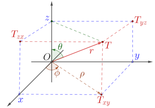
Answer: No. These symbols $\Gamma_{\mu\nu}^\alpha$ are inevitable in tensor calculus, but they are not tensors. Tensors can be covariant or contravariant, depending on how they are transf-ormed from one coordinate system to another, but Christoffel symbols are neither of those.
1. In the image on the right we see the two most popular 3-dimensio-nal coordinate systems on which I will first explain these transformations, and then the Christoffel symbols. The-se are the Cartesian rectangular (Oxyz) and the spherical (Orθϕ) which are al-so orthogonal, so in both the mixed metric tensors gμν are zero:
dℓ² = dx² + dy² + dz², dℓ² = dr² + r²dθ² + r²sin²θ dϕ².
The infinitesimal length dℓ is the same in both coordinate systems, so in the two systems in the figure the length r = OT is also equal. When we fix z = 0, which is θ = π/2, these systems become 2-dimensional Cartesian rectangular (Oxy) and polar (Oρϕ), also both orthogonal coordinates.
2. Tensor calculus is the best thing we have in analysis and analytic geometry precisely because it is based on maintaining invariants, certain values that do not change when the coordinates change. Typical vectors in physics are contr-avariant tensors (rank 1). The displacement vector dxμ, i.e. the position differ-ential, is a contravariant tensor and that is why we write them with superscri-pts.
The gradient of a scalar field, ∇Φ = ∂μΦ is a covariant tensor, and so are the linear functionals (Riesz Lemma) that map vectors to scalars. The metric te-nsor gμν is a doubly covariant, and the inverse gμν is a doubly contravariant tensor. Such quantities, interpreted in certain ways, do not change when wr-itten differently, like ideas in different languages. We use Christoffel symbols to recognize these different writings, and they therefore cannot be tensors.
3. More precisely, any quantity that transforms like coordinate differentials during a change of coordinates is a contravariant tensor. For example, when x1, x2, ..., xn is one entry and y1, y2, ..., yn is another for some of the same quantities (invariants), in the case of a sequence of functions it will be:
$$ y^\mu = f^\mu(x^1, x^2, ..., x^n), \quad \mu \in \{1, 2, ..., n\}, $$ $$ dy^\mu = \frac{\partial f^\mu}{\partial x^\nu} dx^\nu, \quad \nu \in \{1, 2, ..., n\} $$and these are the contravariant transformations. Addition by repeated super-script and subscript is implied.
For example, in the image above, the known functions:
x = r sin θ cos ϕ, y = r sin θ sin ϕ, z = r cos θ,
by differentiation give:
dx = sin θ cos ϕ dr + r cos θ cos ϕ dθ - r sin θ sin ϕ dϕ, dy = sin θ sin ϕ dr + r cos θ sin ϕ dθ + r sin θ cos ϕ dϕ, dz = cos θ dr - r sin θ dθ.
Squaring and then adding and arranging these equalities will give the above (1) intervals, which then represent equal values of dℓ, or invariants. Check!
4. The basis vectors on both sides of these coordinate systems are orthogonal and are often written with a hat on the coordinates. By scalar multiplication of the basis vectors we obtain metric tensors, so:
$$ g_{rr} = \hat{r}\cdot\hat{r} = 1, \quad g_{\theta\theta} = \hat{\theta}\cdot\hat{\theta} = r^2, \quad g_{\phi\phi} = \hat{\phi}\cdot\hat{\phi} = r^2\sin\theta, $$which we read from the upper interval of the spherical system. By adding the basis vectors, we represent all other vectors of the given space by their linear combinations, for example:
$$ \vec{v} = \beta_r \hat{r} + \beta_\theta\hat{\theta} + \beta_\phi\hat{\phi}, $$where βr, βθ and βϕ are scalars (real or complex numbers). However, if we return to the functions and coordinate transformations above, in the more general case it will be:
$$ \vec{y} = B^r\hat{r} + B^\theta\hat{\theta} + B^\phi\hat{\phi}, $$where now Bμ = Bμ(r, θ, ϕ) are functions of coordinates, with the same notati-ons μ ∈ {r, θ, ϕ}. If we continue to work primarily on spherical coordinates, it is convenient to number these basis vectors and write them:
$$ \hat{r} = \vec{b}_1, \quad \hat{\theta} = \vec{b}_2, \quad \hat{\phi} = \vec{b}_3, $$and these Bμ are with indices μ ∈ {1, 2, 3}. Notations are important in tensor calculus. Thus we can write the derivative of the sum of products:
$$ \frac{\partial \vec{y}}{\partial r} = \frac{\partial B^\mu}{\partial r}\vec{b}_\mu + B^\mu\frac{\partial \vec{b}_\mu}{\partial r} $$and similarly for the derivatives of the other two coordinates. Summarizing all three:
$$ \frac{\partial \vec{y}}{\partial \eta^\nu} = \frac{\partial B^\mu}{\partial \eta^\nu}\vec{b}_\mu + B^\mu\frac{\partial \vec{b}_\mu}{\partial \eta^\nu}, \quad \eta = 1, 2, 3. $$These eta are spherical coordinates. Notice something even more important, that the basis vectors are transformed as covariant tensors. Then, the other sums contain the changes of the basis vectors in coordinates.
5. In the case of Cartesian coordinates, for example, $\vec{x} = 2\vec{a}^1 + 3\vec{a}^2 - \vec{a}^3$, there will be a constant displacement (2, 3, -1) at each point in space, two up, three down, and one down, of the basis vectors $\vec{a}^\mu$, and the corresponding derivatives in the coordinates $\partial \vec{a}_\mu/\partial \xi^\nu$ are all zero. However, in the spherical system, not all $\partial \vec{b}_\mu/\partial \eta^\nu$ are zero. We can see this more easily in the polar system (z = 0 and θ = π/2):
$$ x = r\cos \phi, \quad y = r\sin\phi, $$ $$ \vec{b}_r = \frac{\partial x}{\partial r}\vec{a}_x + \frac{\partial y}{\partial r}\vec{a}_y, \quad \vec{b}_\phi = \frac{\partial x}{\partial \phi}\vec{a}_x + \frac{\partial y}{\partial \phi}\vec{a}_y, $$ $$ \vec{b}_r = \cos\phi\, \vec{a}_x + \sin\phi\, \vec{a}_y, \quad \vec{b}_\phi = -r\sin\phi\, \vec{a}_x + r\cos\phi\, \vec{a}_y, $$ $$ \frac{\partial \vec{b}_r}{\partial r} = 0, \quad \frac{\partial \vec{b}_r}{\partial \phi} = \frac{\partial \vec{b}_\phi}{\partial r} = \frac{1}{r}\vec{b}_\phi, \quad \frac{\partial \vec{b}_\phi}{\partial \phi} = -r\, \vec{b}_r. $$We will find something similar for the spherical system, where changes in basis vectors also occur. With the exception of Cartesian coordinates, this means that it makes sense to introduce non-zero summands, and growth coefficients with the basis vectors:
$$ \frac{\partial \vec{b}_\mu}{\partial \eta^\nu} = \Gamma_{\mu\nu}^\alpha \vec{b}_\alpha, \quad \alpha = 1, 2, ... $$These "unknown" coefficients $\Gamma_{\mu\nu}^\alpha$ are precisely the Christoffel symbols. From the above we read:
$$ \Gamma_{\phi\phi}^r = -r, \quad \Gamma_{r\phi}^\phi = \Gamma_{\phi r}^\phi = \frac{1}{r}, $$for polar coordinates. Let's now calculate this for spherical coordinates.
Jacobian » srb
Question: Is there any general instruction on how to transform basis vectors?
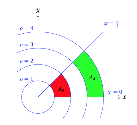
Answer: Yes, there is a “guide” and it is the Jacobian, for example. Si-mply put, if we transform two coor-dinate systems, such as Oxy to Orφ in the image on the left, we add all the increments (basis vectors) of the first system to obtain one by one the increments (basis vectors) of the second. As in the case of ad-ding the force vectors by their co-mponents, the width and height of a parallelogram, to obtain the dia-gonal, the resultant vector. In esti-mating speed, the derivative of the path with respect to time is sought, so here too the increments are the derivatives of the first coordinates with re-spect to the second. That is exactly what the Jacobian does.
1. When transforming basis vectors (usually written with a hat) from Cartesian to spherical coordinates, use the (transposed) Jacobian matrix: $$ \begin{pmatrix} \hat{r} \\ \hat{\theta} \\ \hat{\phi} \end{pmatrix} = \begin{pmatrix} \frac{\partial x}{\partial r} & \frac{\partial y}{\partial r} & \frac{\partial z}{\partial r} \\ \frac{\partial x}{\partial \theta} & \frac{\partial y}{\partial \theta} & \frac{\partial z}{\partial \theta} \\ \frac{\partial x}{\partial \phi} & \frac{\partial y}{\partial \phi} & \frac{\partial z}{\partial \phi}\end{pmatrix} \begin{pmatrix} \hat{x} \\ \hat{y} \\ \hat{z} \end{pmatrix}. $$
Already by the method of such a transformation we recognize that the basis vectors are covariant tensors. Knowing the coordinates (Christoffel I, 3), we find the partial derivatives and form $\hat{b}_\mu = J_\mu^\nu\hat{a}_\nu$ and the matrix equality:
$$ \begin{pmatrix} \hat{r} \\ \hat{\theta} \\ \hat{\phi} \end{pmatrix} = \begin{pmatrix} \sin\theta\cos\phi & \sin\theta \sin\phi & \cos\theta \\ r\cos\theta\cos\phi & r\cos\theta \sin\phi & -r\sin\theta \\ -r\sin\theta\sin\phi & r\sin\theta\cos\phi & 0 \end{pmatrix} \begin{pmatrix} \hat{x} \\ \hat{y} \\ \hat{z} \end{pmatrix}. $$Since the determinant of this matrix is not zero, $|J| = \det(J_\mu^\nu) = r^2\sin\theta$, there is an inverse mapping, spherical to Cartesian basis vectors.
2. Otherwise, the inverse matrix is the adjoint of the given cofactors and divided by the determinant, so J-1 : b → a and J : a → b. It is important that the product of the two is an identity matrix, J-1J = JJ-1 = I. So, the transpose:
$$ J^\top = \begin{pmatrix} \sin\theta\cos\phi & r\cos\theta\cos\phi & -r\sin\theta\sin\phi \\ \sin\theta\sin\phi & r\cos\theta\sin\phi & r\sin\theta\cos\phi \\ \cos\theta & -r\sin\theta & 0 \end{pmatrix} $$we replace the coefficients with cofactors and divide by the determinant:
$$ \frac{1}{|J|}\text{Adj}(J) = \frac{1}{r^2\sin\theta} \begin{pmatrix} r^2\sin^2\theta\cos\phi & r\sin\theta\cos\theta\cos\phi & -r\sin\phi \\ r^2\sin^2\theta\sin\phi & r\sin\theta\cos\theta\sin\phi & r\cos\phi \\ r^2\sin\theta\cos\theta & -r\sin^2\theta & 0 \end{pmatrix}. $$The inverse matrix of the above Jacobian is:
$$ J^{-1} = \begin{pmatrix} \sin\theta\cos\phi & \frac{1}{r}\cos\theta\cos\phi & -\frac{1}{r}\frac{\sin\phi}{\sin\theta} \\ \sin\theta\sin\phi & \frac{1}{r}\cos\theta\sin\phi & \frac{1}{r}\frac{\cos\phi}{\sin\theta} \\ \cos\theta & -\frac{1}{r}\sin\theta & 0 \end{pmatrix}. $$Check the result by multiplication, J-1J = JJ-1 = I. Note that in this case we can guess the inverse matrix, find it without calculation, because the rows of the given matrix are orthogonal intensity vectors of order 1, r and r sin θ, while the columns are the same inverse divided by the determinant. Therefore, the products of the corresponding ones are units, and the incorrect ones are zeros, as required by the unit matrix. In the further search for Christoffel symbols, then the Cartesian system, we also need the translation (r, θ, ϕ) → (x, y, z). However, we will not do this because we know that the required Cartesian symbols are zeros.
3. Let's return to continuation (1). We find the Christoffel symbols of spherical coordinates by calculating the rates of change of the basis vectors in terms of the associated variables:
$$ \frac{\partial \hat{r}}{\partial r} = \frac{\partial}{\partial r}(\sin\theta\cos\phi\, \hat{x} + \sin\theta \sin\phi\, \hat{y} + \cos\theta\, \hat{z}) = 0, $$ $$ \frac{\partial \hat{r}}{\partial \theta} = \frac{1}{r}\, \hat{\theta}, \quad \frac{\partial \hat{r}}{\partial \phi} = \frac{1}{r}\, \hat{\phi}, $$ $$ \frac{\partial \hat{\theta}}{\partial r} = \frac{\partial}{\partial r}(r\cos\theta\cos\phi\, \hat{x} + r\cos\theta \sin\phi\, \hat{y} - r\sin\theta\, \hat{z}) = \frac{1}{r}\, \hat{\theta}, $$ $$ \frac{\partial \hat{\theta}}{\partial \theta} = -r\, \hat{r}, \quad \frac{\partial \hat{\theta}}{\partial \phi} = \frac{\cos\theta}{\sin\theta}\hat{\phi}, $$ $$ \frac{\partial \hat{\phi}}{\partial r} = \frac{\partial}{\partial r} (-r\sin\theta\sin\phi\, \hat{x} + r\sin\theta\cos\phi\, \hat{y}) = r\, \hat{\phi}, $$ $$ \frac{\partial \hat{\phi}}{\partial \theta} = \frac{\cos\theta}{\sin\theta}\hat{\phi}, \quad \frac{\partial \hat{\phi}}{\partial \phi} = -r\sin^2\theta\, \hat{r} - \sin\theta \cos\theta\, \hat{\theta}. $$We obtain the latter by including (2) the inverse transformation:
$$ \hat{z} = \cos\theta\, \hat{r} - \frac{1}{r}\sin\theta\, \hat{\theta} $$in the derivation:
$$ \frac{\partial \hat{\phi}}{\partial \phi} = -r\sin\theta\cos\phi\, \hat{x} - r\sin\theta\sin\phi\, \hat{y} = -r\,\hat{r} + r\cos\theta\, \hat{z} = $$ $$ = -r\, \hat{r} + r\cos^2\theta\, \hat{r} - \sin\theta\cos\theta\, \hat{\theta} = -r(1 - \cos^2\theta)\, \hat{r} - \sin\theta\cos\theta\, \hat{\theta}, $$and that becomes the result written above.
4. We have defined the changes of basis vectors (Christoffel I, 5):
$$ \frac{\partial \hat{b}_\mu}{\partial \eta^\nu} = \Gamma_{\mu\nu}^\alpha \hat{b}_\alpha = \Gamma_{\mu\nu}^1 \hat{b}_1 + \Gamma_{\mu\nu}^2 \hat{b}_2 + \Gamma_{\mu\nu}^3 \hat{b}_3, $$so for μ, ν ∈ {r, θ, ϕ} and given these derivatives, in that order:
$$ \Gamma_{r\theta}^\theta = \frac{1}{r}, \quad \Gamma_{r\phi}^\phi = \frac{1}{r}, $$ $$ \Gamma_{\theta r}^\theta = \frac{1}{r}, \quad \Gamma_{\theta\theta}^r = -r, \quad \Gamma_{\theta\phi}^\phi = \text{ctg}\, \theta, $$ $$ \Gamma_{\phi r}^\phi = \frac{1}{r}, \quad \Gamma_{\phi\theta}^\phi = \text{ctg}\,\theta, \quad \Gamma_{\phi\phi}^r = -r\sin^2\theta, \quad \Gamma_{\phi\phi}^\theta = -\sin\theta\cos\theta, $$and all other coefficients, the Christoffel symbols, are zero. The previous in-dices 1, 2, and 3 here are r, θ, and ϕ, respectively. Let's put them back into more manageable matrices:
$$ \Gamma^1 = \begin{pmatrix} 0 & 0 & 0 \\ 0 & -r & 0 \\ 0 & 0 & -r\sin^2\theta \end{pmatrix}, $$ $$ \Gamma^2 = \begin{pmatrix} 0 & \frac{1}{r} & 0 \\ \frac{1}{r} & 0 & 0 \\ 0 & 0 & -\sin\theta\cos\theta \end{pmatrix} $$ $$ \Gamma^3 = \begin{pmatrix} 0 & 0 & \frac{1}{r} \\ 0 & 0 & \text{ctg}\,\theta \\ \frac{1}{r} & \text{ctg}\,\theta & 0 \end{pmatrix}. $$However, this is not the usual way to find Christoffel symbols.
Hyperspace II » srb
Quesetion: What is the relationship between mentioned Jacobians and metric tensors?
Answer: Let's get to know this (Ja-cobian) connection on simplified, though general, Lorentz transfor-mations (Hyperspace, 3):
$$ \begin{cases} dx_1 = \gamma^{-1}\gamma_0(dy_1 + \beta\, dy_0), \\ dx_0 = \gamma\gamma_0(\beta\, dy_1 + dy_0). \end{cases} $$They are just written a little dif-ferently here. According to the instructions given (Space-Time, page 96), such coefficients can be:
$$ \gamma = \frac{1}{\sqrt{1 - \frac{2GM}{rc^2}}}, \quad \gamma_0 = \frac{1}{\sqrt{1 - \beta^2}}, \quad \beta = \frac{v}{c}, $$where G is the gravitational constant, M is the mass of the gravitational body centered at r = y1 away from the (smaller) body, in free fall in a gravitational field, at time t where y0 = ct is the distance traveled by light in this time. The initial velocity of the falling body is v, and c is the speed of light in vacuum. When M = 0, then γ = 1, so:
$$ dx_1 = \frac{dy_1 - cdy_0}{\sqrt{1 - \frac{v^2}{c^2}}}, \quad dx_0 = \frac{-\frac{v}{c}dy_1 + dy_0}{\sqrt{1 - \frac{v^2}{c^2}}}, $$and these are the well-known Lorentz transformations. Therefore, the above can be called generalized Lorentz transformations.
1. Example. Let's show that:
ds² = γ² dx1² - γ-2 dx0² = dy1² - dy0²,
that these transformations really translate the metric of gravity into the metric of flat space, into the inertial metric.
Proof: Recall, x0 = ct and y0 = ct'. By substituting we find:
$$ ds^2 = \frac{dr^2}{1 - \frac{2GM}{rc^2}} - \left(1 - \frac{2GM}{rc^2}\right)c^2dt^2 = \gamma^2dx_1^2 - \gamma^{-1}dx_0^2 = $$ $$ = \gamma^2[\gamma^{-1}\gamma_0(dy_1 + \beta\, dy_0)]^2 - \gamma^{-2}[\gamma\gamma_0(\beta\, dy_1 + dy_0)]^2 $$ $$ = \gamma_0^2(dy_1^2 + 2\beta dy_1dy_0 + \beta^2dy_0^2)^2 - \gamma_0^2(\beta^2dy_1^2 + 2\beta dy_1dy_0 + dy_0^2) $$ $$ = \gamma_0^2(1-\beta^2)dy_1^2 - \gamma_0^2(1-\beta^2)dy_0^2 $$ $$ = dy_1^2 - dy_0^2. $$And that was what needed to be shown. ∎
2. Here x1 → y1 maps the distances (r) from the center of gravity (of the first and second coordinate systems), so that x0 → y0 are the lengths (ct) that light travels in a given time. We can add the angular coordinates (θ, ϕ) later. The given transformations y → x have a determinant of 1, which is easy to check, and the inverse (x → y) is easy to calculate:
$$ \begin{cases} dy_1 = \gamma\gamma_0\, dx_1 - \beta\gamma^{-1}\gamma_0\, dx_0, \\ dy_0 = -\beta\gamma\gamma_0\, dx_1 + \gamma^{-1}\gamma_0\, dx_0. \end{cases} $$This is useful for us to continue, because we are working with differentials:
$$ dx_1 = \frac{\partial x_1}{\partial y_1}dy_1 + \frac{\partial x_1}{\partial y_0}dy_0, \quad dx_0 = \frac{\partial x_0}{\partial y_1}dy_1 + \frac{\partial x_0}{\partial y_0}dy_0, $$ $$ dy_1 = \frac{\partial y_1}{\partial x_1}dy_1 + \frac{\partial y_1}{\partial x_0}dy_0, \quad dy_0 = \frac{\partial y_0}{\partial x_1}dx_1 + \frac{\partial y_0}{\partial x_0}dx_0. $$We read directly:
$$ \frac{\partial x_1}{\partial y_1} = \gamma^{-1}\gamma_0, \quad \frac{\partial x_1}{\partial y_0} = \beta\gamma^{-1}\gamma_0, \quad \frac{\partial x_0}{\partial y_1} = \beta\gamma\gamma_0, \quad \frac{\partial x_0}{\partial y_0} = \gamma\gamma_0, $$ $$ \frac{\partial y_1}{\partial x_1} = \gamma\gamma_0, \quad \frac{\partial y_1}{\partial x_0} = -\beta\gamma^{-1}\gamma_0, \quad \frac{\partial y_0}{\partial x_1} = -\beta\gamma\gamma_0, \quad \frac{\partial y_0}{\partial x_0} = \gamma^{-1}\gamma_0. $$We have obtained partial derivatives that define Jacobians and metric tensors, each in its own way.
3. Let's define the aforementioned Jacobians:
$$ J^{-1} = \begin{pmatrix} \gamma\gamma_0 & -\beta\gamma\gamma_0 \\ -\beta\gamma^{-1}\gamma_0 & \gamma^{-1}\gamma_0 \end{pmatrix}, \quad J = \begin{pmatrix} \gamma^{-1}\gamma_0 & \beta\gamma\gamma_0 \\ \beta\gamma^{-1}\gamma_0 & \gamma\gamma_0 \end{pmatrix}, $$These map the unit vectors ($\hat{x} = J^{-1}\hat{y}$ and $\hat{y} = J\hat{x}$), respectively:
$$ \begin{pmatrix} \hat{x}_1 \\ \hat{x}_0 \end{pmatrix} = \begin{pmatrix} \frac{\partial y_1}{\partial x_1} & \frac{\partial y_0}{\partial x_1} \\ \frac{\partial y_1}{\partial x_0} & \frac{\partial y_0}{\partial x_0} \end{pmatrix} \begin{pmatrix} \hat{y}_1 \\ \hat{y}_0 \end{pmatrix}, \quad \begin{pmatrix} \hat{y}_1 \\ \hat{y}_0 \end{pmatrix} = \begin{pmatrix} \frac{\partial x_1}{\partial y_1} & \frac{\partial x_0}{\partial y_1} \\ \frac{\partial x_1}{\partial y_0} & \frac{\partial x_0}{\partial y_0} \end{pmatrix} \begin{pmatrix} \hat{x}_1 \\ \hat{x}_0 \end{pmatrix}. $$These two matrices are inverse, J-1J = JJ-1 = I, because γ0²(1 - β²) = 1. The first is secondary, the second is primary, and we need both. Note that we map all differentials and the above transformations to similar, transposed, and replaced Jacobians, respectively:
$$ \begin{pmatrix} dy_1 \\ dy_0 \end{pmatrix} = \begin{pmatrix} \frac{\partial y_1}{\partial x_1} & \frac{\partial y_1}{\partial x_0} \\ \frac{\partial y_0}{\partial x_1} & \frac{\partial y_0}{\partial x_0} \end{pmatrix} \begin{pmatrix} dx_1 \\ dx_0 \end{pmatrix}, \quad \begin{pmatrix} dx_1 \\ dx_0 \end{pmatrix} = \begin{pmatrix} \frac{\partial x_1}{\partial y_1} & \frac{\partial x_1}{\partial y_0} \\ \frac{\partial x_0}{\partial y_1} & \frac{\partial x_0}{\partial y_0} \end{pmatrix} \begin{pmatrix} dy_1 \\ dy_0 \end{pmatrix}. $$The bases are transformed as covariant tensors, however, we transform the coordinates as contravariant tensors.
4. Metric tensors are the coefficients in front of the differential in the interval expression (Example 1). When we switch to the consistent coordinate notation dx4 = idx0 and dy4 = idy0, because differentials are contravariant tensors and we use an imaginary unit for clarity, i² = -1. These expressions will be neater. So, here is how the tensors gμν are related to the Jacobians:
ds² = (dy1)² + (dy4)² =
$$ = \left(\frac{\partial y^1}{\partial x^1}dx^1 + \frac{\partial y^1}{\partial x^4}dx^4\right)^2 + \left(\frac{\partial y^4}{\partial x^1}dx^1 + \frac{\partial y^4}{\partial x^4}dx^4\right)^2. $$We square this and write the shorter derivative notation, ∂j yk = ∂yk/∂xj, hopi-ng that the expressions will be more convenient for further mathematical ope-rations:
ds² = [(∂1y1)² (dx1)² + ∂1y1∂4y1 dx1dx4 + ∂4y1∂1y1 dx4dx1 + (∂4y1)² (dx4)²] + + [(∂1y4)² (dx1)² + ∂1y4∂4y4 dx1dx4 + ∂4y4∂1y4 dx4dx1 + (∂4y4)² (dx4)²],
ds² = g11 (dx1)² + g14 dx1dx4 + g41 dx4dx1 + g44 (dx4)².
We write the same in abbreviated form:
ds² = ∑α ∂μyα∂νyα dxμdxν = gμν dxμdxν,
where it is summed over repeated subscripts and superscripts, here which are μ, ν ∈ {1, 4}. Such expressions give us metric tensors. The procedure is well known and you will easily find other examples (Invariants).
5. In this introduction (2) we have:
$$ g_{11} = \partial_1y^1\partial_1y^1 + \partial_1y^4\partial_1y^4 = (\gamma\gamma_0)^2 - (-\beta\gamma\gamma_0)^2 = \gamma^2, $$ $$ g_{14} = \partial_1y^1\partial_4y^1 + \partial_1y^4\partial_4y^4 = -i(\gamma\gamma_0)(-\beta\gamma^{-1}\gamma_0) + i(-\beta\gamma\gamma_0)(\gamma^{-1}\gamma_0) = 0, $$ $$ g_{41} = \partial_4y^1\partial_1y^1 + \partial_4y^4\partial_1y^4 = -i(\beta\gamma^{-1}\gamma_0)(\gamma\gamma_0) + i(\gamma^{-1}\gamma_0)(-\beta\gamma\gamma_0) = 0, $$ $$ g_{44} = \partial_4y^1\partial_4y^1 + \partial_4y^4\partial_4y^4 = -(-\beta\gamma^{-1}\gamma_0)^2 + (\gamma^{-1}\gamma_0)^2 = \gamma^{-2}. $$This is expected, because ds² = γ² (dx1)² + γ-2 (dx4)², we saw (1st Example).
Perceptions IV » srb
Question: I didn't expect such an unusual example (Hyperspace II) and, seco-ndly, what about the metric tensor and the dot product of basis vectors?

Answer: With all due respect, you will admit that this is a blog with at least some novelty in every answer, without previous announcements from recognized scientific circles, and it is not a school mathematics lesson. I hope this is a place for in-spiration in discovering truths with possible mention, and not for stea-ling ideas. The same will be true wi-th this "scalar product of base vect-ors". I will start explaining metric tensors using perceptions, with the expected continuation (mine or someone else's). The video Metric Tensor is instructive for the explanation I have in mind.
1. It is not possible to globally transform a truly curved space-time (like the or-bit of a planet) into a plane by simply changing coordinates. Intrinsic curvatu-re is a real, inalienable property, similar to the fact that a sphere cannot be fl-attened without stretching or splitting. However, it is possible to have local fl-atness in small regions (free fall, infinitesimal environments), where the effec-ts of gravity would vanish, mimicking flat space. Thus, the transformations fr-om the previous answer are not sustainable for large areas. Nature is telling us that what is possible on a very small scale is not always possible on a large sca-le, and vice versa.
2. The basis vectors $\hat{x}_\mu$ are transformed as covariant tensors, but the coordina-tes $dx^\mu$ are contravariant, so we can write $d\vec{s} = \hat{x}_\mu\, dx^\mu$. Here we mean additi-on by repeated subscripts and superscripts, which here is μ ∈ {1, 4} while x4 = ict = ix0, so the scalar product is:
$$ d\vec{s}\cdot d\vec{s} = ds^2 = \gamma^2 (dx^1)^2 - \gamma^{-2}(dx^0)^2, $$ $$ ds^2 = g_{\mu\nu}\,(dx^\mu)^2(dx^\nu)^2, $$in the notation of the previous answer. The coefficients of the metric tensor are:
$$ (g_{\mu\nu}) = \begin{pmatrix} \gamma^2 & 0 \\ 0 & \gamma^{-2} \end{pmatrix}. $$Therefore, we can write a 2-dim metric tensor in general:
$$ (g_{\mu\nu}) = \begin{pmatrix} \hat{e}_1\cdot\hat{e}_1 & \hat{e}_1\cdot\hat{e}_2 \\ \hat{e}_2\cdot\hat{e}_1 & \hat{e}_2\cdot\hat{e}_2 \end{pmatrix}. $$These are the scalar products of the basis vectors. Here we have the already mentioned y and x coordinates.
3. This refers to physical perceptions, to those realities that we discover throu-gh physical measurements and that occur through interactions. Invariants as well as the status quo, i.e. the sustainability of virtue, are realities (along with observability and truthfulness). Therefore, information perceptions is an im-portant interpretation of the scalar product of vectors. Since it is not possible to list all its important features here, let us emphasize (I explained) only one interesting fact.
What might be visible from the point of view of the micro-world is not so from the point of view of the macro-world, and vice versa. This is also predicted by the law of large numbers of probability theory, in part, but this also includes possibilities that are not expressed by it, including those that are currently un-known to us, or cannot be visible to us. For example, bypassing, i.e. the pheno-menon of micro-particles going to another reality that is not available to us, or similar.
4. The extraordinary accuracy (and even applicability) of mathematical analy-sis when it approximates curved lines by their tangents and locally extends th-em bit by bit to the global is intriguing. Especially, for example, now that we know that some curvilinear coordinates define a non-Euclidean space that we cannot translate into Euclidean space without interruption. In addition to the surface of a sphere, the saddle surface of Lobachevskian hyperbolic geometry has the same property. Although they cannot be aligned without stretching or tearing and are determined for completely different types of geometries, at the infinitesimal level they are equal.
This is another way to misunderstand each other. In addition to the uniquene-ss of each subject's perception, due to the unique information of the percepti-on of the universe, which is a consequence of the uniqueness of the represent-ation of the functional (Riesz Lemma), we also have really different geometri-es of the "same" space-time now and from the point of view of the subjects of the micro and the subjects of the macro-world. To this story of information theory, we should add the reality of infinity, which we in particular cannot physically perceive.
Christoffel II » srb
Question: Can you explain to me the concept of parallel transport and Christo-ffel symbols in tensor calculus?
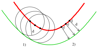
Answer: I'll try. First, consider the description of the parallel curves in this image on the right. If a circle of radius d with center on the upper (red) one slides along the lower (bl-ue) one, then the distance between them is always the same d = const. There are actually two definitions of parallelism, but they are not the goal of this example. More important to us are the vectors on the right that are always perpendicular to the upper one. Vectors perpendicular to them would be tangent to that red circle. The local neighborhood of such displacements, if infinitesimal, in a series of degrees of small displacements Δx, Δx², Δx³, ... will reject everything except the first. Such neglect is the alpha and omega of infin-itesimal calculus and it works.
1. The consequence of this neglect is that we do not see local changes, except global ones. That at such a small quantum level there is no relativity gravity and that hypothetical gravitons have spin 2 so that they cannot interact with individual fermions (spin 1/2), or that the equations of general relativity are written in second-order tensors. Also, (Geodesic) are covariant derivatives of the zero-valued metric tensor:
\[ D_\ell\,g_{\mu \nu } = 0 \]which is an important feature of the Levi-Civita connection. This connection ensures the preservation of lengths and angles (defined by the metric) during parallel transport and makes space-time "locally flat".
2. Covariant derivative is a generalization of the derivative for tensor fields and vectors in curvilinear coordinate systems. It is no different from the ordinary derivative for scalar functions even in flat space, or where there is no differen-ce between the vectors before and after parallel transport. There is also one of the definitions of Christoffel symbols:
$$ D_\ell A^i = \frac{\partial A^i}{\partial x^\ell} + A^k\Gamma_{k\ell}^i, $$where $A^k\Gamma_{k\ell}^i$ determines the change in the vector $A^i$ at different points in sp-ace in the direction of the ℓ-th coordinate.
3. For example, in moving along the x1-th coordinate, the covariant derivative of a vector has Christoffel symbols of zero, as long as the basis vector of that coordinate $\hat{e}_1$ does not change. However, changing the basis vector gives an increment to the derivative, so only the intensity $\|\hat{e}_1\| = e_1$ is important, and we have, in order:
$$ \frac{d(A^1e_1)}{dx^1} = \frac{\partial A^1e_1}{\partial x^1} = \frac{\partial A^1}{\partial x^1}e_1 + A^1\frac{\partial e_1}{\partial x^1}, $$ $$ \frac{1}{e_1}\frac{d(A^1e_1)}{dx^1} = \frac{dA^1}{dx^1} + \frac{A^1}{e_1}\frac{de_1}{dx^1}, $$ $$ \frac{DA^1}{dx^1} = \frac{dA^1}{dx^1} + \frac{A^1}{e_1}\frac{de_1}{dx^1}, $$ $$ \frac{D_1A^1}{Dx^1} = \frac{dA^1}{dx^1} + \frac{A^1}{e_1}\frac{de_1}{dx^1}. $$Because $g_{11} = \hat{e}_1\cdot\hat{e}_1 = (e_1)^2$ and dg11/dx1 = 2e1/dx1, we can write:
$$ \frac{D_1A^1}{Dx^1} = \frac{dA^1}{dx^1} + \frac{A^1}{2(e_1)^2}\frac{dg_{11}}{dx^1}, $$ $$ D_1A^1 = \frac{dA^1}{dx^1} + \frac{A^1}{2g_{11}}\frac{dg_{11}}{dx^1}. $$The contravariant metric tensor gμν and the covariant gμν are inverse matri-ces, and here it is simply g11 = 1/g11 and so on:
$$ D_1A^1 = \frac{dA^1}{dx^1} + A^1(\frac12g^{11}\frac{dg_{11}}{dx^1}). $$In parentheses is the Christoffel symbol (the only one for the sake of simplicity of the example), and D1A1 is the covariant derivative of the one-component ve-ctor A1. The above case is general and more complex.
4. Starting from the previous (2), we expand the covariant derivative to the third-order tensor and find: $$ D_\ell\,A^i_{jk} = \partial_\ell A^i_{jk} + \Gamma^i_{\ell m}A^m_{jk} - \Gamma^m_{\ell j}A^i_{mk} - \Gamma^m_{\ell k}A^i_{jm}. $$
In the case of a metric tensor that has no superscripts, this and (1) give:
$$ D_k\,g_{ij} = \partial_k\,g_{ij} - \Gamma^\ell_{ki}g_{\ell j} - \Gamma^\ell_{kj}g_{il} = 0. $$Let's permute the indices (i, j, k) of this equality into the following three:
$$ \partial_k\,g_{ij} - \Gamma^\ell_{ki}g_{\ell j} - \Gamma^\ell_{kj}g_{i\ell} = 0, $$ $$ \partial_i\,g_{jk} - \Gamma^\ell_{ik}g_{j\ell} - \Gamma^\ell_{ij}g_{lk} = 0, $$ $$ \partial_j\,g_{ki} - \Gamma^\ell_{jk}g_{il} - \Gamma^\ell_{ji}g_{\ell k} = 0. $$Adding the first two and subtracting the third, we get:
$$ \partial_k\,g_{ij} + \partial_i\,g_{jk} - \partial_j\,g_{ki} = $$ $$ = (\Gamma^\ell_{ki}g_{\ell j} + \Gamma^\ell_{kj}g_{i\ell}) + (\Gamma^\ell_{ik}g_{j\ell} + \Gamma^\ell_{ij}g_{lk}) - (\Gamma^\ell_{jk}g_{il} + \Gamma^\ell_{ji}g_{\ell k}). $$Next, we apply the symmetry of the metric tensor index ($g_{ij} = g_{ji}$) and the Christoffel symbols ($\Gamma^\ell_{ij} = \Gamma^\ell_{ji}$), which simplifies this expression:
$$ \partial_k\,g_{ij} + \partial_i\,g_{jk} - \partial_j\,g_{ki} = 2\Gamma^\ell_{ij}g_{\ell k}. $$Multiplying this by the inverse metric tensor, $g_{\ell k}g^{k\ell} = \delta^\ell_\ell$, where we add over k, we find:
$$ \Gamma^\ell_{ij} = \frac12g^{kl}(\partial_k g_{ij} + \partial_i g_{jk} - \partial_j g_{ki}). $$These are Christoffel symbols expressed using a metric tensor.
Conserved » srb
Question:Why are the indices of the metric tensor and the Christoffel symbol symmetric?
Answer: The short answer is, it's because of local symmetry. There are many pitfalls behind understa-nding this seemingly simple phen-omenon. This word symmetry is often used, confusing and needs to be clarified.
In the image on the left, the first figure (a) has three axes of symm-etry and a 120° rotation. The sec-ond figure (b) has two axes of sy-mmetry and a 180° rotation, so the following are the ones where you might notice symmetries yourself. You are looking for those geometric mappi-ngs that will maintain the distances between points. Symmetries of something in general are the preservation of the same thing in different circumstances. For example, science deals with symmetries, the same phenomena in different situations. Another example, the essence of truth is its symmetry.
Symmetry is when different processes lead to the same state, also when diffe-rent paths lead to the same place. In other words, when we add one vector to another and get the same result as when we add the first to the second, $\vec{a} + \vec{b}$ = $\vec{b} + \vec{a}$, also when we add the process A to the process B and get the same st-ate as when we add the first to the second, AB = BA. Such examples show the breadth of the concept of symmetry and reveal one of its deep natures in the law of conservation. That is what we are talking about here, the conservation of Euclidean geometry in small local environments of space-time, as opposed to the global abandonment of that concept. This is an important feature of the Levi-Civita connection and the index symmetry of the metric tensor as well as of the Christoffel symbols.
Energy is not an intrinsic property of matter, but a phenomenon of circumst-ances. Thus, from light to massive bodies, energy depends on the speed of the source, or carrier of motion. Hence its precise measure is the Lagrangian, L = Ek - Ep, the difference between kinetic and potential energy, where the latter is a matter of the wider environment. The principle of stationary action, which is the tendency of nature to maintain this difference, the constant Lagrangian in the motion of a body. Watch this educational video on the topic of Why Ener-gy is ACTUALLY Conserved, in the next image on the right.
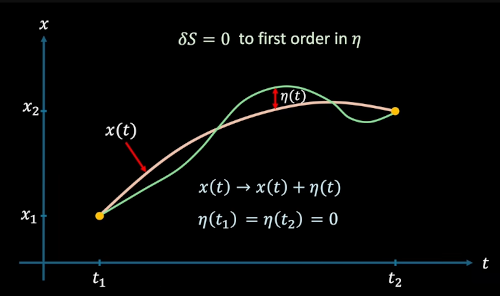
Namely, the action of S on the path x during time t is:
$$ S[x] = \int_{t_1}^{t_2}(E_k - E_p)\,dt, $$where in parentheses is the Lagran-gian which for movement along the abscissa would be:
$$ L = \frac12mv^2 - V(x). $$It is customary to denote the potential, Ep above, in kinematics by the letter V, where m is the mass of the given body and v is its velocity. The green line in the figure is a path that is not realistic because it consumes (the integral acc-umulates) more action than the physical, yellow path. The product of the cha-nged energy and time, dS = Ldt, is what nature wants as little as possible. On that basis, let us consider the following.
Information is in the structure of matter and uncertainty is its essence. These are the reasons why information disappears as soon as it is created and why it is contained in action. This is why the substance is titrating, because its infor-mation is in constant consumption and renewal. On the other hand, we have symmetries, we say laws of conservation, and, on the other hand, we have a spontaneous tendency towards as few actions as possible; stationarity and minimalism. Such come with more frequent realizations of more probable outcomes, simple tendencies towards less informative states and processes. Like some kind of force of rejection from uncertainty that terrorizes nature itself, because without uncertainty one cannot do.
The force F on the path Δx does work ΔE, and the same force is the change in momentum Δp during time Δt, so we have:
$$ \Delta E\,\Delta t = (F\Delta x)\,\Delta t = (\frac{\Delta p}{\Delta t}\Delta x)\,\Delta t = \Delta p\, \Delta x. $$Thus, the action that is the product of the changed energy for a given time is equal to the changed momentum on a given path. According to the uncertai-nty relations, these products are of the magnitude of Planck's constant (h ≈ 6.626×10⁻³⁴ m²kg/s) so, when that small quantity is important, the corresp-onding commutators, of energy with time, or momentum with position, are also important. These are the commutators that define the external informa-tion (In and Out, 3), and with it the presence of an acting force. This force distorts space-time and the actual participant in such a way that the infini-tesimal environment is no longer a flat geometry.
The above-mentioned symmetry of the metric tensor and Christoffel symbols, which arises from treating the small environment as uncurved, comes down to the question of commutativity, which when absent (AB - BA ≠ 0) creates pro-blems for general relativity in quantum mechanics. Incidentally, so does the "accident" with spin 2 gravitons for acting on spin 1/2 fermions.
T-symmetry II » srb
Question: Is time symmetrical? Please give a short and concise answer.
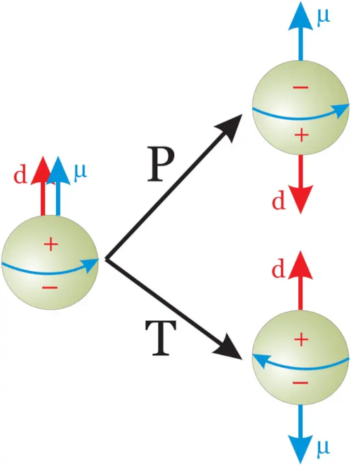
Answer: Depending on the specific circumstances, the answer can be either yes or no. Like in gravity, the question is whether something that falls somewhere must fall anywhe-re. It doesn't have that definite and decisive answer, because a thrown stone falls and then falls to the ground, and the Earth also falls to the Sun, but it never falls.
All the laws of classical physics, not just statistical ones, have time sym-metry, because reversing the direc-tion of time (t → -t) does not chan-ge them. Then again, we have entr-opy, say a vase that falls and breaks and cannot be put back together.
Information theory (mine) has a principle of minimalism that forbi-ds recursion, but also accepts addi-tional dimensions of time, symmetrical to space, that allow it. A recent answer to a similar question (T-symmetry) emphasizes the negation, but let's not for-get the other possibility — as with the orbits of planets.
1. The concept of minimalism is illustrated by global convergence. However, Markov chains themselves demonstrate this sufficiently, so let's take advant-age of this opportunity. The following second-order matrix is stochastic:
$$ A = \begin{pmatrix} 0.7 & 0.4 \\ 0.3 & 0.6 \end{pmatrix} $$because all its coefficients are nonnegative, and both columns sum to one. Its determinant is 0.3, which means that it has an inverse matrix:
$$ A^{-1} = \begin{pmatrix} 2 & -\frac43 \\ -1 & \frac73 \end{pmatrix}. $$This one is pseudo-stochastic. Its column sums are units, but it also has nega-tive coefficients.
2. The characteristic equation Au = λu determines two eigenvalues λ1 = 1 and λ2 = 0.3 then the eigenvectors, say in Euclidean space (2-norm):
$$ u_1 = \begin{pmatrix} \frac45 \\ \frac35 \end{pmatrix}, \quad u_2 = \begin{pmatrix} -1/\sqrt{2} \\ +1/\sqrt{2} \end{pmatrix}. $$They do indeed have the exact characteristic equation, for both vectors, although they are not probability distributions: the simple sums of their coefficients are not units, and furthermore they are not all non-negative. However, in their 2-norm they are unitary:
$$ \|u_1\|_2 = \sqrt{\left(\frac45\right)^2 + \left(\frac35\right)^2} = 1, \quad \|u_2\|_2 = \sqrt{\left(-\frac{1}{\sqrt{2}}\right)^2 + \left(\frac{1}{\sqrt{2}}\right)^2} = 1. $$When we divide them by the sum of the absolute values of their coefficients v1 = u1/(7/5) and v2 = u2/√2, they become the eigenvectors of the same, Av = λv, but they are in a more convenient, 1-norm:
$$ v_1 = \begin{pmatrix} \frac47 \\ \frac37 \end{pmatrix}, \quad u_2 = \begin{pmatrix} -\frac12 \\ +\frac12 \end{pmatrix}. $$Both have an absolute sum of one, but only the first is a probability distribu-tion. I'll explain why such an extensive introduction.
3. Let's try to understand the meaning of the following equation:
$$ Ax_1 = \begin{pmatrix} 0.7 & 0.4 \\ 0.3 & 0.6 \end{pmatrix} \begin{pmatrix} p_1 \\ q_1 \end{pmatrix} = \begin{pmatrix} 0.7p_1 + 0.4q_1 \\ 0.3p_1 + 0.6q_1 \end{pmatrix} = \begin{pmatrix} p_2 \\ q_2 \end{pmatrix} = x_2. $$The distribution x1 with the matrix A transforms into the distribution x2. The second vector is also a distribution, because p2 + q2 = 1 and p2, q2 ≥ 0, but it is closer to the distribution v1, i.e.
|p2 - 4/7| + |q2 - 3/7| ≤ |p1 - 4/7| + |q1 - 3/7|,
whatever the input vector x1 is, as long as it is a distribution. For example, if x1 = (0.8, 0.2)⊤, then x2 = (0.64, 0.36)⊤, while v1 ≈ (0.57, 0.43)⊤. I have given the general proofs earlier.
At the input (x1) there are two possible outcomes, probabilities p1 = 0.8 and q1 = 0.2, which the transmitter A will slightly distort into probabilities p2 = 0.64 and q2 = 0.36. Here we have a 0.7 probability that the first message will be tr-ansmitted correctly and a 0.6 probability that the second will also be transmi-tted correctly. Channel noise (if any) will favor the adaptation of these proba-bilities to the eigenvector v1.
The lesson here is in the approach and convergence of the sequence x1, x2 = Ax1, x3 = Ax2, ... and in general xk+1 = Axk, to the eigenvector v1 of the given matrix. When we have a stochastic process, we also have its law of large num-bers, as in the children's game of "deaf telephones". Channel noise reduces all the initial messages to the same one. We have irreversible global convergence of natural processes.
4. The total information of the present is also distributed to the past, which is why we have reality (duration) and space (storage), in the "desperate" attempt of principled minimalism to give the final word. However, can all this effort of itss be just "pouring the hollow into the empty" (in vain), while memory would sometimes be longer and sometimes shorter; does it grow, fade, disappear, so shrink to reappear? There are ripples in the principle of least action in classic-al physics in its closed cycles too.
Evasion » srb
Question: So, how is it possible to avoid “global convergence” and the flow of time in the same direction?
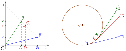
Answer: Adaptation, the adjustme-nt of the state, vector $\vec{x}_k$, for k = 1, 2, 3, ..., to the dominant eigenvect-or $\vec{v}$ of the given process $A\vec{v} = \lambda\vec{v}$ (global convergence), is one of the ways of constant changes towards the status quo. However, changes are also states, all these operators are also types of vectors, so the same laws of minimalism apply to them as well.
1. In the image above left you have the eigenvectors v1, v2 and v3, respectively:
$$ \begin{pmatrix} 0.8 \\ 0.2 \end{pmatrix}, \quad \begin{pmatrix} 0.5 \\ 0.5 \end{pmatrix}, \quad \begin{pmatrix} 0.4 \\ 0.6 \end{pmatrix}. $$I specifically chose them because of their round coefficients and all three have the same eigenvalues λ = 1, for the stochastic matrices A1, A2, A3, respectively:
$$ \begin{pmatrix} 0,9 & 0,4 \\ 0,1 & 0,6 \end{pmatrix}, \quad \begin{pmatrix} 0,6 & 0,4 \\ 0,4 & 0,6 \end{pmatrix}, \quad \begin{pmatrix} 0,4 & 0,4 \\ 0,6 & 0,6 \end{pmatrix}. $$You will notice that only the first column of these matrices changes to change its eigenvector, but both can be changed, so that the eigenvector follows the circle with center C as its tangent vector, on the right-hand side of that figure. We imagine that arbitrary eigenstates, adapting themselves to the processes at the time, follow these eigenvectors.
Now you can easily come up with non-stochastic matrices yourself, either or-dinary real ones or quantum complex ones, with eigenvectors and processes that "run" after them, because global convergence is also their property. That circle on the right can be any conic (line, ellipse, hyperbola), because we have patterns in the orbits of the planets around the sun and symmetry of (at least) three spatial and three temporal dimensions.
2. With the discovery of the spin of quantum particles, we realized that angul-ar momentum can exist without rotation. A wheel, once started, continues to rotate until something stops it, thanks to the conservation of that energy or circular momentum. If not in our environment, then in some pseudo-reality, this possibility of maintaining angular momentum over time is a reality.
It will make their past changeable, moreover very cyclical, much more repeat-able than we see in everyday phenomena (this is a general property of matter waves), but still, always a little different. Over long periods of time, over milli-ons of years, the paths of the planets around the sun shift, and over even long-er periods of time, over billions of years, the solar systems themselves come into being and disappear.
3. There is a situation in special relativity that I wrote about, not in this way, interesting from the point of view of the possible mixing of the past and the future. Otherwise, we know that the light we receive from very distant celestial bodies reveals their past at the time when it was moving towards us. In addi-tion, bodies that are moving have a relatively slower flow of time. When they approach us, they have less and less lag in the past, until the very moment of passing in which the two presents align. Conversely, when they move away, their past that we see is all further away from us.
Time flows more slowly for a body approaching us than for us, and the present is getting closer and closer to us until the moment of passing by, when it equa-lizes, and it appears to be coming from the future. After passing by, that body continues on into the past. It appears as if we have arrived and overtaken the time of such a body.
4. We know from the example of gravity (Holonomy) that small steps can be taken to locally and imperceptibly leave globally straight lines, but perhaps another phenomenon (Adaptation III) is more interesting for the answer here. We know that two consecutive perpendicular polarizers completely stop light, but that another one between them, inclined 45° to both, would allow 1/4 of the ray to pass through all three. Moreover, a long series of very gradual incli-nations between the first and last polarizers will ultimately let all the light through.
Knowing this, we cannot be sure that the present of bodies around us on their way to their futures, converging globally, really all have only one single goal, not to deceive us with their harmony while in fact they are deviating here and there. Such a single goal would be absurd for a theory whose basis is diversity, the assumed general possibilities of choice. What is interesting here is the "av-oidance" of global convergence by means of deceptive immobility, the status quo, either as inertial movement or with a series of inserted obstacles.
|
|
|