|
|
|


The bell » srb
Question: What kind of "regularity" of randomness are you referring to?
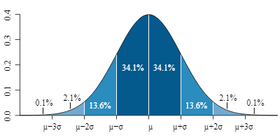
Answer: A probability distribution is a statistical function that describes all possible values and probabilities that a random variable can take in a given range.
The picture on the right shows such a normal, or Gaussian, distribution. It is a "bell curve" with the values of the continuous random variable x along the abscissa. The areas above the abscissa and to the curve are their integral probabilities of the variables that are in the given interval (a ≤ x ≤ b):
\[ \Pr[a, b] = \int_a^b\rho(x)\ dx, \]where ρ(x) is the probability density at the location x, i.e., the density of the variable x, and the ordinates of the curves are ρ = ρ(x), where the probability density is:
\[ \rho(x) = \frac{1}{\sigma\sqrt{2\pi}}e^{-\frac12\left(\frac{x - \mu}{\sigma}\right)^2}. \]The densest probabilities are around the variable μ, which we call expectation and which in general amounts to:
\[ \mu = E[X] = \int_{-\infty}^{\infty} x\rho(x)\ dx, \]The second letter σ in the picture is the root of the mean square deviation from the mean value, the square of which we call the variance:
\[ \sigma^2 = E[(X - \mu)^2] = \int_{-\infty}^{\infty} (x-\mu)^2\rho(x)\ dx. \]Dispersion is generally the name for scattering around some values, so this sigma is sometimes called dispersion. The picture shows that the variables from μ - σ to μ + σ contain 68.2 percent of all Gaussian distribution probabilities. Variables from μ - 2σ to μ + 2σ will pick up approximately 95.4 percent of such probability, and those from μ - 3σ to μ + 3σ contain almost all the probabilities of this normal distribution.
The Gaussian distribution was called "normal" after scientific publications in the 19th century that revealed many natural phenomena with almost regular deviations from the mean. The idea of "normal variability" was popularized by the naturalist Galton in his 1889 paper "Natural Inheritance." However, financial and some other phenomena do not follow a completely normal distribution but can be more or less settled.
However, the central limit theorem, which holds for sequences of independent random variables with the same probability distribution, with finite expectation and variance, states that the sampling distribution of those means will be normal when the sample size is large enough. Regardless of whether the population has a normal, Poisson, binomial, or any other distribution, the sampling distribution of the same mean will be normal. Hence the wide applicability of the Gaussian distribution.
When X1, X2, X3, ... a series of random variables from the same probability space, with equal and mutually independent probability distributions and finite μ and σ, we observe the n-th partial sum:
Sn = X1 + X2 + ... + Xn.
We easily see that Sn has expectation nμ and variance nσ². Standardized random variable:
\[ Z_n = \frac{S_n - n\mu}{\sigma\sqrt{n}} \]when n → ∞ tends to a normal distribution with mean 0 and variance 1. This is the content of the aforementioned central limit theorem, and it is routinely used in statistics in this way.
Let's note that forming a standardized random variable Zn in this case, we add uniform independent distributions Xk in the value Sn, which then become new random variables. First, we thereby define a third random variable Zn with predefined mean μ and variance σ². Second, we arrive at it through a homogeneous distribution, otherwise with the greatest information of all on the given interval.
Namely, when the possible outcomes are not of equal chance and happen more often, more likely, such an occurrence is less informative, less uncertain. What we create by forming Zn is the opposite of that, a uniform chance distribution of a given dispersion σ. It will therefore become Shannon's maximum information. However, we know from before (Extremi, 1.7) that for the given finite variance σ² the greatest information \(S \le \ln(\sigma\sqrt{2\pi e})\) has precisely the normal distribution and only it.
This informational explanation (proof) of the central limit theorem is also an explanation of the cause of the deviation of natural phenomena from the normal distribution, which can be more or less settled. Namely, nature will spontaneously strive for states of less information. She does not like equality and tries to find order in differences.
Chebyshev » srb
Question: What are the "regularities" of non-normal distributions?
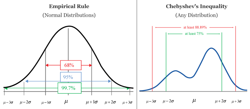
Answer: Chebyshev's inequality is a more general version of the percent density restriction than those given for normal distributions. In this picture, the left graph sketches the density accumulations of the Gaussian distribution, and the right one is the general Chebyshev's. About 75 percent of all chances fall between μ - 2σ and μ + 2σ values of random variables, and close to 89 percent are in the range from μ - 3σ to μ + 3σ.
The following theorem establishes Chebyshev's inequality with proof for the general case of expectation μ. Earlier I gave proofs of this inequality, especially for continuous distributions and discrete, both for expectations μ = 0.
Theorem. For an arbitrary distribution of random variables from the set X, with mathematical expectation μ = E[X] and variance σ² = V[X] = E[(X - μ)²], for an arbitrary real number r > 0 the probability inequality holds:
\[ \Pr[|X - \mu|\ge r] \le \frac{\sigma^2}{r^2}. \]This is Chebyshev's inequality.
Доказ: In the general case (∀μ ∈ ℝ) is:
\[ \sigma^2 = \int_{-\infty}^{\infty}(x-\mu)^2\rho(x)\ dx \ge \] \[ \ge \int_{-\infty}^{\mu - r}(x-\mu)^2\rho(x)\ dx + \int_{\mu + r}^{\infty} (x-\mu)^2\rho(x)\ dx \] \[ \ge \int_{\infty}^{\infty} r^2\rho(x)\ dx + \int_{\mu + r}^\infty r^2 \rho(x)\ dx \] \[ = r^2\left(\int_{-\infty}^{\mu - r}\rho(x)\ dx + \int_{\mu + r}^\infty \rho(x)\ dx\right) \] \[ = r^2\Pr[|X - \mu|\ge r], \]and hence the aforementioned Chebyshev's inequality. ∎
For example, in some class a test was given where the average student score was μ = 60 out of a 100 possible points with a dispersion of σ = 15 percent. We wonder how many students exceeded or fell short of the average by more than r = 30 percent of points:
\[ \Pr[|X - 60| \ge 30] \le \frac{15^2}{30^2}. \]That is a quarter, or 25 percent of the students.
It is easy to understand why the application of Chebyshev's inequality goes far beyond statistical analysis. It is an important tool for finding deviations from the "regularity of randomness," detecting false data, setting norms, modeling in general, and even machine learning.
Chebyshev's inequality reveals to us that there is also a probability limit at the distance r from the mean value μ. It is a limit that decreases by means of constant central forces — with the square of the distance. I have written a lot (locally, privately) about this connection between the abstract space of probabilities and physical space-time, which is mostly consolidated in the script Information Coupling (1.2.4 Conic Sections).
In short, it can be proved that whatever constant central forces, like Newton's gravity and also Coulomb's electricity, must decrease with the square of the distance. Then they move the charges along the lines of the conic so that the stroke that connects the center and the charge in equal times covers equal surfaces. When there is no force, the conic is a straight line. When the force is attractive, the conics are ellipses and parabolas, and if the force is repulsive, the conic is a hyperbola.
Chebyshev's inequality tells us about the repulsive force of uncertainty whose boundary lines of probability decrease with the squares of the distances given (expectations μ and dispersions σ) of abstract probability spaces.
Conics » srb
Question: How do you use Chebyshev's inequality?
Answer: In various ways. Its use in information theory and physics is a bit unusual for my purposes, so I'll elaborate on that.
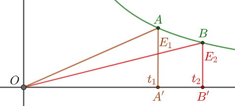
In the picture left, we imagine that the point A → B moves along the hyperbola, the green curved line. Its two projections on the abscissa are A' and B', and the ordinates of the height are E1 and E 2 at distances t1 and t2 respectively, from the origin O. If the hyperbola yx = const, i.e., Et = const, then the areas of the triangles OA'A and OB'B are equal because the products of the legs of those right triangles are equal.
1. We imagine that the point charge is driven by the force F⋅x² = const. from the center O along the hyperbola y = 1/x. The work of the force on the road requires energy dE = F⋅dx, and hence eliminating the force and integrating we find E⋅x = const. Тhen we calculate that the path x = ct is such that the light travels in time t. Briefly stated, this is an explanation of the above picture using a repulsive central force that decreases with the square of the distance and moves the charge along a hyperbolic path.
2. Another explanation would be emphasizing that physical action is a product of energy and time and is the "equivalent" of information (there is no physical information without action, nor is there physical action without the transmission of information). Then the product of the legs OA'⋅A'A = OB'⋅B'B of these right triangles due to their equal surfaces, now produced by energy and time, tell us about the constancy of the overall action over the duration of time. We equate the law of conservation of information with forces from the center that decrease with the square of the distance.
Even if the whole universe is in the picture, with the Big Bang at O, the OA duration of about 13.8 billion years, and the present AA', it will be a review in accordance with this theory of information. Reality is that which lasts, which is subject to the law of conservation, and therefore has an increasingly long history and a decreasingly ongoing present. Information is all reality with uncertainty at its core.
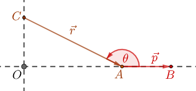
3. The image on the right shows angular momentum, the vector \(\vec{L} = \vec{r}\times\vec{p }\). It is the vector product of two vectors:
\[ \vec{r} = \overrightarrow{CA}, \quad \vec{p} = \overrightarrow{AB}, \]of position and momentum, with θ oriented angle between them.
We know that this product is a vector perpendicular to the plane of the direction factor vector of the right-hand rule, with intensity L = rp sin θ, i.e., by the area of the triangle ABC. In the absence of forces, the angular momentum is kept the same while the material point slides uniformly along the abscissa, A → B. Analogously, the area of a triangle is always the same because it is a semi-product of constant height CO and base AB.
The absence of force and the preservation of the momentum of the cosmic present, as in the previous paragraph, would mean that the law of conservation still applies, also that there is an increasingly long history, but that the present does not lose information. That would slightly devalue principled minimalism, and although interesting, it is not my priority interpretation.
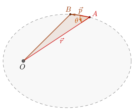
4. The picture on the left inspires one, perhaps even more attractive idea than the previous one, which is also less of a priority for me. General Kepler's second law states that for central forces that decrease with the square of the distance, the stroke joining force and charge will sweep equal areas at equal times.
The area of the triangle OAB is constant, and then the analogy with the universe and all its history becomes obvious.
The intensity current AB of the "momentum" vector \(\vec{p}\) is drawn along the focal ellipse at the point O. It is pushed towards the center O by the environment full of indeterminacy; we can also say it is attracted by the force of probability where its indeterminacy is rarer, i.e., where certainty is greater, it changes the saturation of its information periodically in revolutions around the source of certainty.
5. The above elliptic model of constant action is more acceptable when we look at it locally. Such groups of information exist in the present with a past of a constant total amount and with what we are seeing right now, with more or less uncertainty depending on the observer's point of view. It makes sense when we consider that the "same" news is not the same surprise for everyone.
I have already explained that different observers, for example, because of their own uniqueness and information as a fabric of space, time, and matter, cannot perceive reality equally. Reality therefore does not exist as an absolute. That is why the elliptical model of interactions is so much more worth considering. I take it seriously, but not too seriously.
La Ola » srb
Question: Can you just replace the distance x = ct with the time t it takes light to travel that distance at speed c?
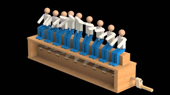
Answer: Yes, I think, above all, in the spread of radiation, vacuum expansions. These are gauge bosons: photons, gluons, gravitons, and other massless "particles" that would move at the speed of light. And let me remind you, time (almost) stands still for such observers, and what is perceived is actually continuities of that kind of particle in the time flow of the observer. In addition to all this, the present is advancing towards the future at the speed of light and that's it.
That way these models (Conics) are very faithful. I build these expressions so that uncertainties push objects, phenomena, or processes out of themselves with some virtual actions (let's not forget that states are vectors, and they are also linear operators), so we get processes of attraction by greater certainty. For example, consider the ripple of a group of people as in the image above to the right and the attached link.
A group of people may pass a package from hand to hand, but it doesn't arrive until the whole group has. Thus, light can appear to travel "faster than light" through a cloud of cesium atoms, as researchers at the Princeton Institute have observed (New Jersey, 2000), finding light to emerge even before entering such a cloud. However, careful analysis reveals that it is a "wave within a wave," a phase of the wave, which, like mail being added within a group of people, will not reach its destination before the group.
Many who watched the wheels turning on the films of different speeds could notice that depending on the frequency of the spinning images, they rotate opposite to the movement of the vehicle. Depending on the relative time course of the process, such a process may have a "wave within a wave," a phase of the wave traveling in the opposite direction of the wave itself. Unlike the illusion of a video, a real perception will have real consequences.
Thus, we can assume that a virtual sphere from a negatively charged electron, from the point of view of a positive charge, has the opposite phase flow from the wave itself. In the eventual interaction, she will "give" him such a negative momentum, and the result is the attraction of the negative with a positive charge. In the direct phase with the wave, there will be a repulsion effect, as in the case of charges of the same sign.
The opposite direction of rotation of the wheel, propeller, and other alternating repetitions can also be seen in the accelerated shots. Selected, accelerated slide change frequencies will show the opposite direction of motion, demonstrating the attractive force of a center of greater certainty from an environment of slower time flow. In the previous answers, it is understood that the environment of increasing uncertainties is "livelier" in the sense of faster frequencies of events and faster flow of time, and therefore repulsive.
This would not contradict my earlier description (Current), if we accept that electrons at rest have virtual spheres of photons whose phases move opposite to the direction of the wave. These relative observations of charges of the same name in mutual rest, in relative motion would be seen with phases moving in the direction of the wave. At rest the equal charges would attract each other, but as soon as they were set in motion (in either direction), they would repel each other and continue to repel each other.
Slit in Time » srb
Question: Are you claiming that light reaches the subject simultaneously from multiple layers of time?
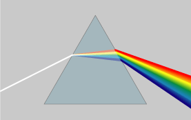
Answer: Yes, but it is not a property of light alone (Conics). The linked image on the left is Newton's prism when he (1665) resolved the "particles" of white light into the elementary seven colors. On, from top to bottom: red, orange, yellow, green, blue, indigo, and violet. As they were gravitationally attracted differently from the particles of the transparent medium (Newton believed), the colors refracted differently.
It became a historic mistake when in 1801 Thomas Young devised a new "double aperture" experiment, believing that he had once and for all proven the wave nature of light, instead of a particle. Also in Newton's "particle proof," as well as the next one, let's note that action at a distance is tacitly implied. Here it is, the penetration of light (information) from multiple layers of time into the same present of the observer.
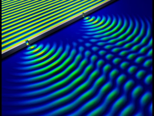
In the picture on the right we see a representation of Young's experiment (Double-slit). A wave of light encounters a flat obstacle that has two narrow openings through which the light leaks. At the output we have two waves that will interfere and leave a diffraction image, alternating bands of stronger and weaker intensities, on the eventual curtain.
We are not dealing here with the "quantum mystique" of that experiment, which I rationalized earlier by handing over the information at the aperture; if one tried to measure through which aperture the light particle passes, it would lose its wave effect. Instead, we focus on the "actions at a distance" of the interference process itself. The superposition of waves does not come from the joining of the very present, simultaneity, because even the smallest distance is separated by time due to the limitation of the speed of information transmission.
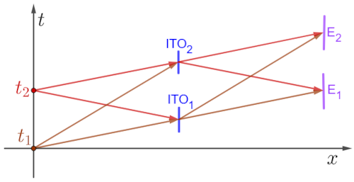
Pictured on the left is a sketch (Time Slit) experiment, Imperial College in 2023. Then, for the first time, interference similar to Young's double aperture, but of light emitted at different times, was explicitly demonstrated t1 and t2 in the distance of Δt = t2 - t1, lasting a few femtoseconds (1 fs = 10-15 s).
On the vertical axis is time (t), and on the horizontal axis is distance (x). On two occasions (t1 and t2), light is sent to the indium tin oxide plate ITO from which the surfaces of mobile phone screens are made. It has, for this occasion, the fantastic property of being able to alternately transmit and reflect light within a few fs time intervals (Δt). Then the interference of previous and future light occurred, recorded on the screen (E1 and E2) in two different moments (Slit in Time).
If we have established this kind of "action at a distance" (distinguish it from quantum entanglement), we see the slowing down of light passing through optically denser media as interference between the light and the material through which it passes. The speed is adjusted, averaged with the speed of the waves of that material, and the light of a higher frequency (blue) is more susceptible to this, and it is refracted more than the red, which oscillates more slowly. The light of higher frequencies, more lively, prefers to adapt to slower flows, and in the following it would be a story about principled minimalism.
Information reaches the subject simultaneously from multiple layers of time, but that time depth Δt is actually very shallow. Therefore, the particle wave is not large; its packet is limited by the capacity of the indeterminacy of its position. Greater uncertainty of place means greater wavelength λ and less uncertainty of momentum p = h/λ; we can now say, according to larger entrainments from the environment. However, due to the high speed of light and its even greater square, the force that decreases with the square of the distance x = ct, given our usual t, has a very shallow memory range.
Torque » srb
Question: Can a moment of force be associated with information?
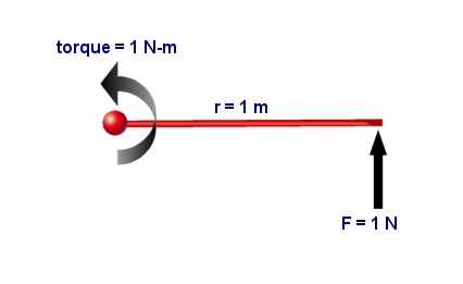
Answer: In the picture on the right, we see the moment of force, torque, which is also called the total torque of the coupling, just the moment. It is equal to the vector product of the position vector r and the force F:
τ = r × F,
intensity τ = rF⊥ = rF sin θ, where θ = ∠( r, F) angle between position and force vectors. The answer to the question is expectedly positive, primarily due to the assumption of the ubiquity of information.
1. As the angular momentum vector is L = r × p, where the linear momentum is the vector p = mv and m is the mass multiplied by the velocity vector v, so the time derivative:
\[ \frac{\mathbf{L}}{dt} = \mathbf{r}\times\frac{d\mathbf{p}}{dt} + \frac{d\mathbf{r}}{dt}\times \mathbf{p} = \mathbf{r}\times\mathbf{F} + \mathbf{v}\times\mathbf{p} = \mathbf{r}\times\mathbf{F}, \]because velocity and linear momentum are parallel, so v × p = 0. Therefore, the moment of force is the change of angular momentum with time. Like we connected the linear moment with probability (Conics, 3), so the connection with information as a resistance to principled minimalism. While L is the result expression of spontaneity, the τ is its change, which it resists.
2. Let's find the moment of force for the central forces. We use the notation r0 as usual \(\hat{r} = \vec{r}/r\) for the unit vector of the position vector r and the variance σ²k0 let's put proportional to gravitational GMm, with k0 = 1:
τ = r × F =
\[ = \mathbf{r} \times \frac{\sigma^2}{r^2}\mathbf{r}_0 = \frac{\sigma^2}{r^2}\mathbf{r} \times \mathbf{r}_0 = 0, \]dL/dt = τ = 0, L = const.
Therefore, there is no torque (momentum of force) exerted by the central force, and the angular momentum (momentum of momentum) is constant.
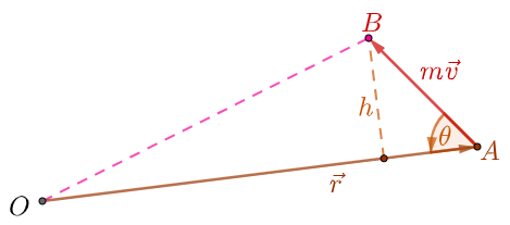
3. In the picture on the left is the center of force in point O. Consider the consequences of conservation of angular momentum:
L = const.
The small area change of triangle OAB is dS = rh/2 = rv sin θ dt/2, and hence dS/dt = rv sin θ = L/2m. This is the Kepler's second law. In equal times, the radius vector of the charge will cover equal areas, simply due to the conservation of angular momentum.
4. We view physical space-time, the points A(x, y, z, ct), as an abstract space of probability positions of random variables, and using only, for now, Chebyshev inequality, we find strong analogies with the behavior of bodies in gravity. In the same way, the moment of force is related to probability and is connected to information. If there are no further questions, this answers the above.
Orbits » srb
Questions: I can't be surprised at the ease with which you handle these formulas and how persistent you are to explain to us how it's all a "scientific joke." Do you really think that "frivolity" is all that you write about?..
Answers: What I'm writing to you about is less than the tip of the iceberg, so sometimes I miss something supposedly serious. It happens to me, but writing seriously on the networks then entails endless bitter discussions with "experts" who can convince you with unprecedented energy and enthusiasm that you are wrong. That's why "You didn't understand well; I'm not interested in science, but science fiction" is my saving statement. I will now answer your second question, about orbits.
1. Sticking to the aforementioned variance analogy with gravity, σ² = GMm, where G is the gravitational constant, and M and m are the masses of the larger and smaller body, below is:
F = GMm/r² = σ²/r²,
where r is the distance between the centers of the two masses. From F = ma it follows σ² = mar², where a is the acceleration, and especially σ² = mv²r when a = v²/r is centrifugal acceleration (Information Coupling, 3.2.2 Spinning Top). Of course, you can replace the above equality of variance and gravity with say a proportion, but this idea will remain the same.
2. Centrifugal force balances the celestial bodies with gravity, so it is:
a = v²/r = GM/r²
\[ v = \sqrt{\frac{GM}{r}}. \]It is the speed of a body (planet) in orbit around mass M, at a distance r from its center. Let's derive Kepler's Third Law: the squares of the orbital periods T of the planets are directly proportional to the cubes r of the semi-major axes of their orbits.
3. Kepler's third law states that T² = r³ for planets, where T is the orbital period measured in years and r is the distance from the Sun, measured in astronomical units (AU). This is true for Earth, where T = 1 year and r = 1 AU. Since the circumference of the circle is 2πr = vT, it will be:
\[ \sqrt{\frac{GM}{r}} = \frac{2\pi r}{T}, \] \[ T^2 = \frac{4\pi^2}{GM}r^3. \]This is the general scale that Kepler's Third Law is about. However, for the mass M of the Sun, the value of the constant 4π²/GM = 2.96×10⁻²⁵ s²/cm³, and there are 31 million seconds in a year and 1 AU = 1.3×10¹³, so that value constant is one, in units of years and astronomical units, as Kepler set.
4. Variance replacement, σ² = GMm, is also possible in expressions for kinetic Ek and potential Ep the energy of a body of mass m in the gravitational field of mass M:
\[ E_k = \frac12mv^2, \quad E_p = - \frac{GMm}{r}, \]where v is the velocity of the body in orbit when it is at a distance r from the center of gravity. Unlike potential energy, kinetic energy cannot be negative, and for any elongated ellipse, it is always Ek + Ep ≤ 0. Here the equality holds if the velocity is:
\[ v_e = \sqrt{\frac{2GM}{r}} \]escape speed from orbit. For Earth's gravity, this speed at a distance of r kilometers from the center is ve = 894/√r [km/s]. Therefore, to take off from the surface of the earth, r = 6378 km, and an initial velocity ve = 894/√6378, or 11.19 km/s is required.
***
From all this we see that the units of variance are σ² let's say kg m3 s-2, or it is the dimension of the coefficient k0 in the expression σ ²k0 = GMm when is the variance σ² dimensionless.
Polar » srb
Question: What does orbital motion look like in polar coordinates?
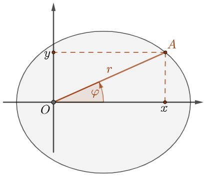
Answer: In the picture on the left, the point A(x, y), Cartesian rectangles, is written as A(r, φ) in polar coordinates. Then it is:
x = r cos φ, y = r sin φ,
\[ r = \sqrt{x^2 + y^2}, \quad \varphi = \text{arctg}\frac{y}{x}. \]
Everything we do next uses these transformations. Here's how.
1. Let's also include the equations of motion of Cartesian coordinates:
r = x i + y j, F = Fx i + Fy j,
where i and j are the orthos (unit vectors) of the Cartesian abscissa and ordinate (x and y axes). This first one, r = (x, y), is the radius position vector, and the second F = (Fx, Fy) is the force vector.
2. Force is the product of mass and acceleration, so we have:
\[ \mathbf{F} = m\ddot{\mathbf{r}} = m(\ddot{x}\ \mathbf{i} + \ddot{y}\ \mathbf{j}) = F_x\ \mathbf{i} + F_y\ \mathbf{j}. \]When this is the central force, directed towards the origin O, then (F = |F|):
\[ F_x = \mathbf{F}\cdot \mathbf{i} = -F\cos\varphi = -F\frac{x}{\sqrt{x^2 + y^2}}, \] \[ F_y = \mathbf{F}\cdot \mathbf{j} = -F\sin\varphi = -F\frac{y}{\sqrt{x^2 + y^2}}. \]Hence, with F(x, y) = F, the equations of motion:
\[ \ddot{x} = - \frac{xF(x,y)}{m\sqrt{x^2 + y^2}}, \quad \ddot{y} = - \frac{yF(x,y)}{m\sqrt{x^2 + y^2}}. \]The substitution in the above easily checks them.
3. Let us denote the unit vectors with er = r/r along the radius and with eφ perpendicular to it. So, we have:
r = r er, er = cos φ i + sin φ j,
\[ \dot{\mathbf{r}} = \dot{r}\mathbf{e}_r + r\dot{\mathbf{e}}_r, \quad \dot{\mathbf{e}}_r = r(-\sin\varphi\mathbf{i} + \cos\varphi\mathbf{j})\dot{\varphi} = \mathbf{e}_\varphi \dot{\varphi}, \] \[ \dot{\mathbf{r}} = \dot{r}\mathbf{e}_r + r\dot{\varphi}\mathbf{e}_\varphi. \]The first addition, item, is the radial component of the speed, from the origin straight outside, and the second addition is the speed's transverse (orthogonal, tangential) component; it goes along the circle's line, perpendicular to the radius.
4. To find the acceleration equations, we differentiate this velocity:
\[ \ddot{\mathbf{r}} = \ddot{r}\mathbf{e}_r + \dot{r}\frac{d}{dt}\mathbf{e}_r + \frac{d}{dt}(r\dot{\varphi})\mathbf{e}_\varphi + r\dot{\varphi}\frac{d}{dt}\mathbf{e}_\varphi = \] \[ = \ddot{r}\mathbf{e}_r + \dot{r}\mathbf{e}_\varphi \dot{\varphi} + (\dot{r}\dot{\varphi} + r\ddot{\varphi})\mathbf{e}_\varphi + r\dot{\varphi}\frac{d}{dt}\mathbf{e}_\varphi. \]The derivative of the unit angle vector is:
\[ \frac{d}{dt}\mathbf{e}_\varphi = \frac{d}{dt}(-\sin\varphi \mathbf{i} + \cos\varphi \mathbf{j}) = -\cos\varphi \dot{\varphi}\mathbf{i} - \sin\varphi\dot{\varphi}\mathbf{j} = -\mathbf{e}_r \dot{\varphi} \]and because of that:
\[ \ddot{\mathbf{r}} = \ddot{r}\mathbf{e}_r + \dot{r}\mathbf{e}_\varphi \dot{\varphi} + (\dot{r}\dot{\varphi} + r\ddot{\varphi})\mathbf{e}_\varphi - r\dot{\varphi}^2\mathbf{e}_r = \] \[ = (\ddot{r} - r\dot{\varphi}^2)\mathbf{e}_r + (2\dot{r}\dot{\varphi} + r \ddot{\varphi})\mathbf{e}_\varphi. \]At the same time:
\[ 2\dot{r}\dot{\varphi} + r\ddot{\varphi} = \frac{1}{r}\frac{d}{dt}(r^2\dot{\varphi}). \]So the acceleration equations are:
\[ \ddot{\mathbf{r}} = (\ddot{r} - r\dot{\varphi}^2)\mathbf{e}_r + \frac{1}{r}\frac{d}{dt}(r^2\dot{\varphi})\mathbf{e}_\varphi. \]The first addition, in parentheses, is the radial component of the acceleration, and in the second, the factor of the unit vector eφ, is the tangent component.
5. In summary, the results of the 3rd and 4th derivations are the velocity and acceleration equations:
\[ \dot{\mathbf{r}} = \dot{r}\mathbf{e}_r + r\dot{\varphi}\mathbf{e}_\varphi \] \[ \ddot{\mathbf{r}} = (\ddot{r} - r\dot{\varphi}^2)\mathbf{e}_r + \frac{1}{r}\frac{d}{dt}(r^2\dot{\varphi})\mathbf{e}_\varphi \]
We obtained these equations in polar coordinates for the central force, without considering the intensity of the force.
6. We continue with central forces, products of mass m and these accelerations, f(x, y) = f(r):
\[ m\ddot{\mathbf{r}} = m(\ddot{r} - r\dot{\varphi}^2)\mathbf{e}_r + \frac{m}{r}\frac{d}{dt}(r^2\dot{\varphi})\mathbf{e}_\varphi = f(x,y)\mathbf{e}_r \]and the component of the force perpendicular to the radius is zero:
\[ \frac{m}{r}\frac{d}{dt}(r^2\dot{\varphi}) = 0 \ \Rightarrow \ r^2\dot{\varphi} = s = \text{const}. \]This constant s also talks about the conservation of angular momentum and Kepler's second law, which we have already seen (Torque) in a slightly different way. Further, putting dφ/dt = s/r², we have:
\[ m(\ddot{r} - \frac{s^2}{r^3}) = f(x,y). \]Two coordinates x and y can be replaced by one vector r = (x, y), so we can say that this is a second-order differential equation with only one variable.
7. From these equations and Newton's second law, we find the law of conservation of energy:
\[ \int m\dot{\mathbf{r}}\cdot\ddot{\mathbf{r}}\ dt = \int \dot{\mathbf{r}}\cdot(m\ddot{\mathbf{r}})\ dt = \int \mathbf{F}(\mathbf{r})\cdot\frac{d\mathbf{r}}{dt}\ dt = \int \mathbf{F}\cdot d\mathbf{r}, \] \[ \frac12m|\mathbf{r}|^2 - \int \mathbf{F}\cdot d\mathbf{r} = \text{const}. \]On the left, the first of the previous, the integral is calculated as kinetic energy. Energy is subtracted from it as the work of the force on the road, which is V(r) potential energy in the case of conservative forces (where the work on the road depends only on the endpoints). Then we have a potential, the function V such that the equality F = -∇V is valid, and the previous equality can be written:
\[ \frac12m|\mathbf{r}|^2 + V(\mathbf{r}) = E \]where E is the total constant energy of the system. It is the sum of the kinetic and potential energy of the system. Compare this with the slightly different derivation of the same in the previous answer (Orbits, 4).
8. Here, with a different procedure, we arrive at the same result as in the book Information Coupling (1.2.4 Conic Sections), and finally, Binet's formula (1.4), which we will also perform consistently in this way. Let's put the change of radius in the known transformation:
\[ \frac{du}{d\varphi} = \frac{du}{dt}\frac{dt}{d\varphi} = \frac{1}{\dot{\varphi}}\frac{du}{dt}, \quad u = \frac{1}{r}. \]On such u, we find the first and second derivatives by time:
\[ \frac{du}{dt} = \frac{1}{\dot{\varphi}}\left(\frac{-1}{r^2}\right)\dot{r} = - \frac{\dot{r}}{s}, \] \[ \frac{d^2u}{d\varphi} = \frac{dt}{d\varphi}\frac{d}{dt}\left(\frac{-\dot{r}}{s}\right) = - \frac{1}{s\dot{\varphi}}\ddot{r}. \]Written differently, this gives:
\[ \ddot{r} = -s\dot{\varphi}\frac{d^2u}{d\varphi^2} = -s(su^2)\frac{d^2 u}{d\varphi^2} = -s^2u^2\frac{d^2u}{d\varphi^2}. \]Again \(s = r^2\dot{\varphi} = \dot{\varphi}^2/u^2\), whence \(\dot{\varphi} = su^2\), then the force equation (6) we write:
\[ m\left(-s^2u^2\frac{d^2u}{d\varphi^2} - \frac{1}{u}(su^2)^2\right) = f(1/u), \] \[ \frac{d^2u}{d\varphi^2} + u = -\frac{f(1/u)}{ms^2u^2}, \]and that is the Binet formula just mentioned (2S = s).
9. In the mentioned book (Sprega Informacija, p. 24), it was shown that Binet's formula, otherwise the equation of the trajectory in the polar system, is the equation of the conic (19th problem). The general equation of the conic in the polar system is included there:
\[ \frac{1}{r} = \frac{1 + \varepsilon \cos\varphi}{\varepsilon d}, \]with eccentricity ε and directrix d and shown to satisfy Binet's formula so that the force is:
\[ f(r) = \frac{4ms^2}{\varepsilon d}\frac{1}{r^2}, \]therefore, such that it decreases with the square of the distance. According to the previous (Orbits), where the variance was σ² = GMm, now σ² = 4ms²/εd. Hence GM = 4s²/εd.
Most of the planets of the solar system have very small eccentricities ε of approximately circular orbits. Earth has eccentricity ε = 0.0167. Its distance to the Sun at aphelion (around July 4) is about 3.3% greater than at perihelion (around January 3). Comets have a very high eccentricity, close to 1, and very elongated ellipses of orbits.
10. Let's do here the reverse of the solution in the book; let's start from Newton's gravitational force and the abbreviation σ² = GMm; we solve the equation:
\[ -f(r) = \frac{GMm}{r^2} = \frac{\sigma^2}{r^2}, \] \[ \frac{d^2u}{d\varphi^2} + u = \frac{\sigma^2}{ms^2}, \] \[ u = C_1\cos\varphi + C_2\sin\varphi + \frac{\sigma^2}{ms^2}. \]We easily check that this is the solution of that differential equation; differentiating twice and adding with u, and given that the derivative σ²/ms² is zero. This can also be expressed in the following form:
\[ u = \frac{1}{r} = C\cos(\varphi - \alpha) + \frac{\sigma^2}{ms^2}, \]where we phase-shifted the angle φ → θ = φ - α, for some arbitrary α. All three integration constants C, C1, and C2 are also arbitrary. Hence:
\[ \frac{ms^2}{\sigma^2r} = 1 + \frac{Cms^2}{\sigma^2}\cos\theta, \] \[ \frac{\ell}{r} = 1 + \varepsilon \cos\theta. \]This is the conic of polar coordinates, directrix ℓ and eccentricity ε. As we know, if the eccentricity ε = 0, this curve is a circle; when 0 < ε < 1, it is an ellipse; when ε = 1, it is a parabola; and if ε > 1, it is then a hyperbola. The directrix and eccentricity are:
\[ \ell = \frac{ms^2}{\sigma^2} = \frac{s^2}{GM}, \quad \varepsilon = \frac{Cms^2}{\sigma^2} = \frac{Cms^2}{GMm} = \frac{Cs^2}{GM}. \]The planets of the solar system mostly move in ellipses (ε close to zero) that are approximately circular. From this solution and Kepler's first law, we know that the Sun is at their focus. Based on Kepler's second law, that the radius r in constant times (let it be time T) covers the same surfaces (surface sT/2), applied to the entire ellipse, we find that s/2 is equal to the area of the ellipse divided by the period of revolution.
Otherwise, the area of the ellipse with the semimajor a and minor b is πab. Hence, the time it takes a planet to go around the Sun, the one revolution, is T1 = 2πab/s. It is also ℓ = a(1 - ε²), b² = a²(1 - ε²), and ℓ = s²/GM, so we calculate:
\[ T_1^2 = \frac{4\pi a^2b^2}{s^2} = \frac{4\pi a^2b^2}{GM\ell} = \] \[ = \frac{4\pi a^2b^2}{GMa(1 - \varepsilon^2)} = \frac{4\pi a^2b^2}{GMa(b^2/a^2)} = \frac{4\pi a^3}{GM}, \] \[ \frac{T_1^2}{a^3} = \frac{4\pi}{GM}. \]We obtained Kepler's third law, that the squares of the orbital periods of the planets are directly proportional to the cubes of the semi-major axes of their paths, in a way slightly different from the previous one (Orbits, 3). This ratio does not depend on the choice of the planet (it does not depend on the mass m), but only on the mass of the Sun (mass M).
***
This is the "poetry" of mathematics that we admire and trust in astronomy. All the above calculations have long been known to physics, including the use of the substitution σ² = GMm, except that we give it such a different label and do not call it a variance. By the way, privately in similar expressions, I denote the variance with σ² = GM in units of kg m²/s², in addition to the above, and I often use a coefficient in front to leave that term σ², for probability, dimensionless.
We would say that physics is more "accurate" than mathematics because it seeks concrete confirmation of "truths," and yet, due to the need for experimental confirmations, it is more "inaccurate" than mathematics because it is blind to other "truths." I'm privately on the latter, stretching the idea of "action equivalent to information" to the max in seeking its breaking point. Until further notice, that story "holds water"—through the spontaneous striving of nature towards "order in diversity." For now, the mentioned "poetry" of mathematics in astronomy is just another proof of such a concept.
Graph » srb
Question: Are you talking about "nature's spontaneous tendency toward order in diversity" as a principle of this theory?
Answer: No, the principle is to strive for less action, information, or greater probability. Behind that comes the movement towards diversity and order. I'll explain one more time.
1. The uniform probability of the distribution is the most uncertain, contains the most information (Extremi, 1.5), and it is easy to understand intuitively, without formulas. Namely, when some outcome is more likely than the rest, it happens more often, and surprises are rarer. Therefore, spontaneous developments towards diversities.
2. We have fewer options when we know more precisely what to do. That's what the rules are for: to reduce uncertainty and wandering, to be more efficient, or not to bother with dilemmas about what to do next and why. A similar thing happens with the general spontaneous flow towards order. In physics, at the starting point of everything is the principle of least effect, but equally as such, but less understood as such, is the adherence of matter to the laws of nature.
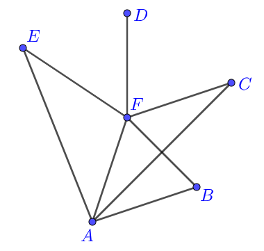
3. Graph theory also has many examples of principled minimalism and the mentioned consequences, not to mention only theoretical physics. Take, for example, the image above on the right, a graph with six nodes A, B, C, D, E, and F, with eight links AB, AC, AE, AF, BF, CF, DF, and EF. We need up to two links to connect any two nodes. Node F has five, A four, nodes B, C, and E have two each, and node D has only one link.
When we connect each of the n = 6 nodes to each other, the number of links is:
\[ N = \binom{n}{2} = \frac{n(n-1)}{2} = 15. \]That's a lot more than the eight in the picture, but there would be a transition from each node to any other in just one step. However, links would dominate the graph. It would be a situation like the acquaintance of each of us in the world (there are eight billion people today) with every other person. All those immediate acquaintances are not possible, firstly because of the limits of our memory, and looking deeper, because of principled minimalism.
The way of natural savings is precisely the minimalism of information that arranges us in such a way that anyone can connect with anyone on the planet in just six steps (Six degrees of separation). For an even larger number of nodes (eight billion), that number of steps would be greater than six, but the number of links would not grow as fast as if each were directly connected to each other. It is a better way of building telephone exchanges, electricity transmission lines, and computer networks, which builders come to intuitively.
4. This efficiency of distribution, starting from equal links that lead to the inequality of nodes, we understand with probability itself through the construction of the network. Namely, let's imagine that at one moment we are building a network of peer-to-peer links and peer-to-peer nodes. Then every node has the same number of links, and all links are equally likely. If we add a new link following the previous one, we will disturb that balance, and the equality of the link will cause the inequality of their ends.
If a node has multiple links, such as node F in a given image, the chances are that the new node would be directly connected to F than to A are 5 : 4, and in relation to the others even less, in relation to D as much as 5 : 1. If we convert these chances into one distribution of Probabilities, we will get:
\[ \Pr = \begin{pmatrix} A & B & C & D & E & F \\ \frac{4}{16} & \frac{2}{16} & \frac{2}{16} & \frac{1}{16} & \frac{2}{16} & \frac{5}{16} \end{pmatrix}. \]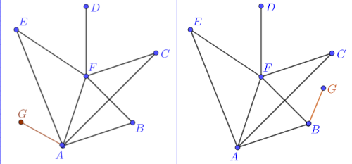
Above is the label of the node, and below it is the probability that its link will be chosen. For example, in the first picture on the left, it would be Pr(A) = 4/16. In that second picture, Pr(B) = 1/8. Nodes with more (equal) connections will have them even more compared to the others by expanding the network. The new distributions are, if A is selected and when B is selected:
\[ \begin{pmatrix} A^* & B & C & D & E & F & G \\ \frac{5}{18} & \frac{2}{18} & \frac{2}{18} & \frac{1}{18} & \frac{2}{18} & \frac{5}{18} & \frac{1}{18} \end{pmatrix}, \] \[ \begin{pmatrix} A & B^* & C & D & E & F & G \\ \frac{4}{18} & \frac{3}{18} & \frac{2}{18} & \frac{1}{18} & \frac{2}{18} & \frac{5}{18} & \frac{1}{18} \end{pmatrix}, \]and the other four are easy to match. Equality of flows leads to inequalities of stations. For example, this is the case in the free market of money, goods, and services, whose wealth is driven by the inequality of the owners.
5. Calculations based on probability suggest that the principle of minimalism is behind the unequal distribution of links by nodes, and yet official science has not come to that for now. This means that the answer to the above question is not very simple, so here is an additional explanation. Namely, the very "striving for order in diversity" would lead the network to one node with all links and all other nodes with only one each.
This does not happen, because then we would have equality of (almost) all nodes, and nature does not really like equality (see 1). So, if we reverse the matter and assume minimalism, then as a consequence we get efficiency in order and diversity. To make matters even more complicated, there are no completely equal links.
Saturation » srb
Question: When the details pile up, there is oversaturation and nightmare, and there is less and less "order in diversity," right?
Answer: No, because the broader concept of trees is a forest. Just look at the previous answer (Graph, 4) with the enormous complexity of the resulting graphs by building and capturing the vision that finds regularity in their layering.
That first distribution Pr starts with six outcomes (A, ..., F), and the next one has seven (A, ..., F, G). The outcomes of the first can be divided into 16 elements, the second into 18. By adding one link to the network, one new node is obtained, but a distribution with two more elementary outcomes is created. Probability divisors, by link steps, grow much faster than numerators, because all the lower ones (denominators) are increased by two, while only one of the upper ones (numerators) is increased by one. There are more and more outcomes and smaller and smaller probabilities.
On the one hand, we have the Borel-Cantelli lemma, which says (of course the order of these probabilities converges) that with total probability 1, it can be realized just finally a lot of options. Therefore, infinitely many outcomes become irrelevant. Indeed, the process of adding new ones will create lonely nodes, each with one connection to someone from the network. When there are more of them, there is a greater chance that a new link will be attached to one of them, so that there will be fewer isolated ones. This goes along with the remark that nature does not want equality, nor such loners, which is why it will avoid the situation of a single node with all links.
On the other hand, if there is an infinite sequence of these additions, which is therefore "only" countably infinite and of cardinality ℵ0, in cases of adding many links at once in steps, a continuum 𝔠 = 2ℵ0 choices. Namely, how 0,abc... is the binary notation of a positive real number less than one, where the digits a, b, c, ... form an infinite series of zeros or units, and there is a continuum of such records; this means that the set of choices cannot be placed in a set of links or nodes. Namely, because the continuum is an infinity of a higher order than countable infinity.
Similarly, we further imagine an infinity of 2𝔠 of a higher order than the continuum 𝔠, to conclude that there are no infinities at all or that there are also infinitely many of them. I stand by the latter, holding to the objectivity of randomness as well as consequences, like additional dimensions of time. Especially then, it can be said that we are also like this, limited in finite perceptions that manage to grasp so many infinities, so how then can we doubt entities, as separate subjects, at higher levels of complexity.
However, we do not have to go so far as to note that an almost infinite number of molecules of a substance have, for our understanding, a proper mass, or velocity, volume, and the like. Nature is very generous in giving meaning to "oversaturated." Some of everything we recognize well, we can only think about a lot, and most of the phenomena of nature we have not been able to imagine until now.
Afterlife » srb
Question: Is there life after death?
Answer: A seemingly silly but frequently asked question that I understand is aimed at the subject of information theory, eager for a meaningful and written answer. There is no such thing as a stupid question until a stupid answer.
Here I define reality by means of three criteria: perceptibility, maintenance, and truthfulness. The first is that subject B can perceive object A, that C can perceive B, ... that X can perceive something from the previous sequence, from which, in the case of "continuity of possibilities," the occurrences of A, B, C, ..., and X are candidates for being mutually "real." There is no need for constant, incessant mutual stares, nor opportunities for such, but for the existence of only chances for some of the previously mentioned interactions.
From what has been said, duration follows, which I emphasize no less than as a law of conservance. The model is the law of conservation of energy, whose forms change but the quantity remains, which I then see as a consequence of the conservation of action, and I derive this from the conservation of information. In this way, the first and second conditions of "reality" are almost equivalent. Similarly, hence the third accuracy condition. Nature is not able to lie (the demonstrably impossible will not happen), so the physical action only applies to truths.
However, not everything that exists is "real." There are also "fictions," at least of the kind we can perceive (objects of imagination), which last like Pinocchio as long as our memories of him last, and which in that sense are truly character. In short, what does not meet all three criteria of "reality," but we will consider "existing," I call "fiction." Next, we should define "life after death," which is a concept that, frankly, I have not yet dealt with.
To the question, "Is there life after death?" I like to ask, "And do you have life before death?" when you are so interested in the latter. Or, as Socrates once said: "There really is no death, because when there is us, there is no death, and when there is death, there is no us." If I come up with something better, I'll let you know.
Quandary » srb
Question: Why does the possibility of choosing make us nervous?
Answer: Both the lack and excess of alternatives will make us restless, depending on the nature of the circumstances. By putting uncertainty at the center of action, information theory shows some more than the known explanations.
1. A living being, relative to the inanimate substance of which it is composed, has additional options that I sometimes call "vitality." It is "trapped" in the personal belt between the lower and upper amount of choices that make it peaceful. The death drive draws the bottom, i.e., the principle of minimalism, upper curiosity, that is, the need to maintain the amount of uncertainty (information) it possesses. Defined differently, above the lower limit we are held by the desire for freedom, and below the upper limit by the fear of the unknown.
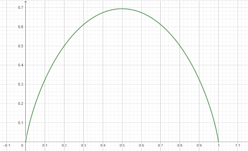
2. In the picture on the right is the graph of the function:
y = -x⋅ln(x) - (1 - x)⋅ln(1 - x).
The abscissa and ordinate are:
x ∈ (0, 1), y ∈ (0, ln 2),
probability and information, respectively. The highest value of the function y = ln 2 ≈ 0.69 is achieved with the value x = 0.5.
3. Practically, we are looking at a random event that can happen, with probability 0 < p < 1 represented on the abscissa, or will not happen with probability q = 1 - p. The information is the binary probability distribution, that is, the superposition of states, the ordinate. Uniform distribution has the greatest information when being is equal to not being.
We have greater uncertainty of options with more even chances. Those choices require significant efforts of will from us, and these also need considerable vitality, greater defiance to the principled minimalism of information, i.e., enhanced actions. When we rise above the upper limit of comfort, nervousness and cracking are natural responses. When the choices to be or not to be also become some special uncertainties, things get even more complicated and require greater defiance of the principle of minimalism, the spontaneous tendency of nature towards less information.
4. Let's examine the binary distributions P and Q of the probabilities sums, say p1 + p2 = 1 and q1 + q2 = 1, which are the outcomes of again the third binary distribution A, sum of probabilities a1 + a2 = 1. With probability a1, something from P will happen, and with probability a2, something from Q will happen. We assume that Pi is an event from P of probability pi and Qj is an event from Q with probability qj, where indices i, j ∈ {1, 2}. Combined, we thus make a new probability distribution a1p1 + a1p2 + a2q1 + a2q2 = 1. That's easy to check. All these probabilities are positive real constants.
5. Let's say P1 ∈ P and Q1 ∈ Q desired outcomes in some token game (Gain). When P1 happens, the player gets a token and loses a token if P2 happens. Also, in the game Q, if Q1 occurs, the player gains a token, and loses a token when Q occurs 2. When p1 > p2, then player P statistically wins with a series of moves (sometimes he loses, sometimes he wins, but in a longer series he wins). Also, in the case of q1 > q2, player Q will statistically win with a series of moves; otherwise, he loses.
6. The combined, cascading case, in which A1 ∈ A and P1, will mean winning tokens with probability a1 p1. Also, the token gain is when A2 and then Q1 happen, which will be with probability a2 q1. So the token gain is if:
a1p1 + a2q1 > a1p2 + a2q2,
a1p1 + (1 - a1)q1 > a1(1 - p1) + (1 - a1)(1 - q1),
a1(p1 - q1) + q1 > 1 - a1(p1 - q1) - q1,
a1(p1 - q1) + q1 > 0,5.
When this inequality is reversed, the game is losing. In Parondo's game, which I mentioned in the last blog (link here), it is not q1 + q2 = 1, and the trick in it is the excess situations of numbers that are not divisible by three.
7. I was asked an interesting question once when I hardly understood what the interlocutor actually meant, but now is an opportunity to renew it. When the distribution of two outcomes, say these A, activates the distributions P or Q, whether and why the information is dependent on the information P and Q?
I consider the answer to be expected, but I will explain it. Three particular upper distributions have Shannon information:
I(P) = -p1⋅ln p1 - p2⋅ln p2,
I(Q) = -q1⋅ln q1 - q2⋅ln q2,
I(A) = -a1⋅ln a1 - a2⋅ln a2.
The Shannon information of pooled, linked distributions is:
I(A; P, Q) = -a1p1⋅ln a1p1 - a1p2⋅ln a1p2 - a2q1⋅ln a2q1 - a2q2⋅ln a2q2 =
= -a1p1⋅(ln a1 + ln p1) - a1p2⋅(ln a1 + ln p2) - a2q1⋅(ln a2 + ln q1) - a2q2⋅(ln a2 + ln q2)
= -a1⋅(p1 + p2)⋅ln a1 + a1⋅(-p1⋅ln p1 - p2⋅ln p2) - a2⋅(q1 + q2)⋅ln a2 + a2⋅(-q1⋅ln q1 - q2⋅ln q2)
= -a1⋅ln a1 - a2⋅ln a2 + a1⋅(-p1⋅ln p1 - p2⋅ln p2) + a2⋅(-q1⋅ln q1 - q2⋅ln q2),
I(A; P, Q) = I(A) + a1⋅I(P) + a2⋅I(Q).
The information of the merged distributions is equal to the mean information of the outcome distributions increased by the information of their selection.
8. This type of extension is easily generalized to a distribution A with outcomes A1, ..., Am probability a1, ..., am, positive real numbers sum to one. Each individual k = 1, ..., m outcome Ak activates one distribution Pk whose outcomes are Pk1, ..., Pkn probability pk1, ..., pkn. This is how we define a pooled two-step concatenated distribution with mn probabilities:
a1 p11, a1 p12, ..., am pmn.
It consists of positive (maybe non-negative) real numbers that add up to one. That has Shannon's information:
I(A; P1, ..., Pn) = I(A) + a1I(P1) + ... + amI(Pm),
where I(P1), ..., I(Pm ) information of the resulting distributions.
9. We have also reached the bonus for the answer to the above question. In the development of the universe, or its parts of separate systems, from the uncertainties that are the past, an average is taken according to new probabilities (if A is a distribution) whose information added to the previous average becomes a new value. The trend of a similar repetition of the present does not go into a more informative future if I(A) does not increase, and the outcomes of the new probabilities do not favor the more informative Pk distributions (uniform). In this way, the universe can develop into a more certain one.
Collapse II » eng
Question: Can you explain wavefunction collapse to me?
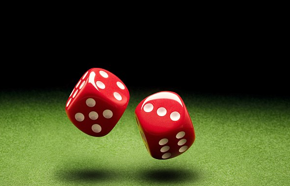
Answer: Quantum mechanics has the term "wave function collapse," which it also calls state vector reduction — for the description of the transition of the wave function from the superposition of several eigenstates to one of them due to the interaction with the environment.
This interaction is an observation and represents the essence of quantum mechanics measurements that relate the wave function to classical observables such as position and momentum. Collapse is the first of two processes by which the states of quantum systems evolve over time, the second being the continuous evolution governed by the Schrödinger equation. I further explain the "collapse" from the point of view of my information theory, and it should be known that it is still enigmatic in official physics.
1. Let's consider the mentioned collapse using probability distribution. After throwing two dice, as in the picture above on the right, one of the 36 pairs of numbers from the set S = {(1,1), (1,2), ..., (6,6)} will fall. That the events, say, (4,3) and (3,4), are different, we can determine by repeating the roll many times and, when the dice are fair, noting that a particular event occurs in approximately 1/36 cases. There is one and only one outcome from the set S, and then we consider this distribution before throwing it as a superposition and its collapse — the outcome.
2. Collapse is an act of simultaneity. Shannon's information of the outcome is equal to such (the amount of uncertainty) of the prior distribution, and it is one expression of the law of conservation of information. Also, the overall uncertainty of a state of the present does not change; it is conserved before and after the collapse of the superposition. For example, in the case of quantum entanglement (I'm talking about what is unknown to official physics), two particles move apart so that they have, say, zero total momentum or spin. The simultaneous delivery of information in one place declares the second in another.
3. What we think of as "the present" is actually a multiplicity of individual and elementary presents. For example, a virtual sphere of photons expanding around an electron is inherently simultaneous but is not seen as such by other observers. The simultaneity of the system in motion is not such for a relative observer. Due to their fragmentation and multiplicity, we look at various simultaneities in the macro world averaged, approximately, and this confuses us for now.
Every relative movement has a special simultaneity, and we know that everything around us moves and moves in relation to everything around us. That's why we have no choice but to count on approximations of the "present" and on the limitations of such rounding. However, you should know that it is only an approximate estimate that can sometimes let us down.
4. The analysis of "nervousness due to the possibility of choosing" (Quandary, 8) is also an explanation of the effect of future uncertainties on the phenomena of the time flow. Superpositions, often of few outcomes (at least two), labeled there as A distributions, which collapse into A1, A2, ..., respectively, with probabilities a1, a2, ... realizations are present in further occurrences of corresponding distributions indicated there by the above indices P¹, P², ... in a process that is constantly ongoing for each of the present in their own ways.
5. In addition to all this, the collapse of the wave function also points us to the reality of uncountable infinity; here's how. Like the distribution of multiple options that realized only one of them (1), and the possibly infinite steps of the time flow (4) that keep only one of the options at a time, they resemble real number entries in the base b ∈ {2, 3, ...}, which is usually binary (b = 2) or decimal (b = 10).
Looking at the real numbers from the interval (0, 1), of which there are infinitely many continuum (uncountable), each can be written in the unique forms 0,b1b2..., with an infinite sequence of digits bk ∈ {0, 1, ..., b}, and they give us ways to "perceive" uncountable infinity with countable infinity (Sets). Cut that number to the first n ∈ ℕ digits; they will be able to write bn different numbers, i.e., values. When the number of digits grows indefinitely (n → ∞), their sequence will become countably infinite (ℵ0), and the number of values will become uncountably infinite (continuum, 𝔠).
In this way, with mathematical perceptions of truth, at first glance the finite present, alone allows us insights into the infinite. The first of the criteria of "reality," its observability, is realized. The second is permanence, which is implied for infinities as parts of mathematics. Truths are indestructible, unlike falsehoods. And the third criterion of "reality" is truthfulness, in this case obviously fulfilled. Since continuums are types of reality, so are the additional dimensions of time.
Retrospective » srb
Question: How do you explain the effect of the present on the past?
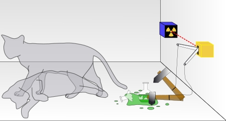
Answer: You're probably thinking of Heisenberg's famous sentence (1926) that "by measuring an ele-ctron, we actually shape its previ-ous path as well," or of the thought experiment "Schrödinger's cat.".
1. Vectors represent quantum states. However, operators are, again, vectors, and quantum processes belong to the types of quantum states. Therefore, the collapse, i.e., the outcome of the wave function, will also be the collapse of the quantum process. At the same time, "electron measurement" as an authentic pheno-menon differs from the "cat" thought experiment, where the law of large numbers (probability theory) significantly cancels the consequences of uncertainty.
In the micro world, measurement is a dramatic phenomenon. The observa-tion, whether it is a collision or the emission of a photon, in the macro world would have the character of a disaster for both sides of the communication. Such a large change in the sender's information would significantly reduce its uncertainties so that we could easily see an increase in its certainty, including better definitions of its previous states. This is exactly what happens in the micro world on a micro level, which for them is not as "micro" as we see it.
2. When X denotes a vector space with scalar components Φ (real or complex numbers), then X* is the label of its dual vector space. Dual is the space of li-near mappings (Information Coupling, Functionals), of vectors X into scalars Φ. Therefore, sums of products are also dual vector spaces; they are spaces of n-tuples of numbers (scalars), so according to what has been said, they can be interpreted as both states and processes. They are forms of information of perception.
The form of the sum of products is recognizable:
Q = a1b1 + a2b2 + ... + anbn
as a scalar (inner) multiplication of vector-strings, here a = (a1, a2, ..., an) and b = (b1, b2, ..., bn). We write it algebraically Q = a⋅b and quantum-mechanical Q = ⟨a, b⟩, no matter if the scalars are real, but this second insight is more pr-ecise when the scalars are complex numbers. The second, quantum way corre-sponds to the micro world and real, elementary simultaneities. That informa-tion of perception, therefore, by the very act of creation, exhausts some uncer-tainties of the participants, including those from their recent past.
3. Dual space X* of vector space X, scalar Φ of complex or real numbers, is the space of linear functionals on X of the label ℒ(X, Φ). When X and Y are finite-dimensional vector spaces, then ℒ(X, Y) denotes the space of linear mappings X → Y whose dual space is ℒ(X, Y)*. Spaces ℒ(X, Y)* and ℒ(X*, Y*) have the same dimensions, and as such they are isomorphic, then there is a linear bijection between them.
The inner (scalar) product of the space ℒ(X*, Y*) can be defined with ⟨A, B⟩ = Tr(A*B). It is the trace of the mapping product A, B ∈ ℒ(X, Y) among which the first factor is adjoined. From Riesz's representation theorem, for every linear mapping A ∈ ℒ(X, Y)* it follows that A : X* → Y*. I mention this to readers who are possibly familiar with dual vector spaces, for which the topic does not need to be elaborated.
It is enough for us to note that there is a wide range of usage of the concepts of states and processes within their interpretations using vectors. In the micro world, the spaces are Hermitian, with complex coefficients and real eigenva-lues, and in other cases, symmetric mappings are sufficient as well as stocha-stic matrices (Markov chain).
4. Stochastic matrices are those whose columns are some probability distri-butions and are therefore good for explaining choices (Quandary). Let's say:
\[ \begin{pmatrix} p_1 & q_1 \\ p_2 & q_2 \end{pmatrix}\begin{pmatrix} a_1 \\ a_2 \end{pmatrix} = \begin{pmatrix} a'_1 \\ a'_2 \end{pmatrix}, \]shorter written Sa = a', when all their columns are some probability distri-bution, is one such example. The stochastic matrix does not have to be sy-mmetric (equal to its transpose) but will always have λ = 1 for one of the eigenvalues with eigenvector v = (v1, v2)⊤, so that Sv = v, which is some distribution (non-negative coefficients sum to one). Here it is:
\[ \mathbf{v} = \begin{pmatrix} \frac{q_1}{q_1 + p_2} \\ \frac{p_2}{q_1 + p_2} \end{pmatrix}, \]which is easy to verify. When this matrix is symmetric, we will have p2 = q1 and v = ( 1/2, 1/2)⊤. The composition of constant stochastic matrices forms a Markov chain, and with Sna → v, when n → ∞, if and only if det(S) ≠ 1.
In other words, when the Markov chain generator (matrix S) does not lose its signal, it is not an isometry; the chain does not become a "black box." It then does not make a series of transformations after which the input message is not known from the output message. Applied to the development of events, we are in a position to read the input message. The further back we look into the past, the more obscure we see it. The older the incoming message is, the greater its uncertainty is. From this, we would believe the future of the universe is more and more certain.
5. From this point of view, the present from which we see the past and not the future, with the assumed uncertainty in the development of the universe, our present and future determine the past. Namely, we arrived here where we are, and we could have been something else, so the present is a witness, and the choices made, a creator of its past.
|
|
|