July III 2025 (Original ≽)

In mathematics, physics, and science in general, vectors are quantities that contain multiple numbers (scalars). They are elements of vector spaces and, for example, points of metric spaces. The following topics provide interpre-tations of vectors, starting with the states of quantum systems and then exte-nding to other natural phenomena. Linear mappings are also vectors, and so are the processes of their interpretation. When we simplify them, we express vectors in terms of oriented lengths and then in terms of intensity, direction, and course.

Volume II » srb

Question: How do you link the value of information to volume?

Answer: This is a formal relations-hip. For example, (Figuration), the smallest particles do not have a "shape", which already speaks of the connection between informa-tion and space. There is a theorem (Joseph Fourier, 1822) that says that almost any function (read: trajectory) can be arbitrarily acc-urately approximated by a fraction of any other such function, which is a mathematical admission of the position about the non-existence of shapes in the smallest particles. Then this justifies their other uncertainties, among many, and the connection of information wi-th spatial forms.

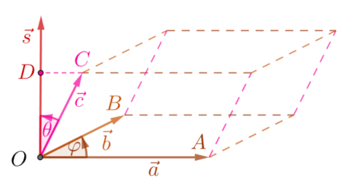
1. In the figure on the right, in the plane, say Oxy of the rectangular Cartesian coordinate system, there are two vectors \(\vec{a}\) and \(\vec{b}\) between which the angle φ is oriented so that they span a parallelogram of area equal to the intensity of the vector:

\[ \vec{s} = \vec{a}\times \vec{b}, \quad |\vec{s}| = ab\sin\varphi, \]

where a and b are the intensities of the given vectors in the plane. This "surf-ace vector," otherwise the vector product of two vectors, or the outer product of vectors, is perpendicular to the plane with the direction determined by the "right-hand rule," i.e., right screw, which means the aforementioned "surface" is also an oriented quantity. When the angle between the vectors is obtuse, the sine will be negative, as will that value.

We write the same vectors using projections onto the coordinate axes and using orthonormal vectors (unit vectors of those axes), so the area vector is:

\[ \vec{s} = \vec{a}\times \vec{b} = (a_x\vec{i} + a_y\vec{j})\times (b_x\vec{i} + b_y\vec{j}) = (a_xb_y - a_yb_x)\vec{k}. \]

This is the form in which we recognize the commutator of a vector (Polygon):

\[ [\vec{a}, \vec{b}] = a_xb_y - a_yb_x = ab\sin\varphi. \]

It is further closely related to the concept of information in the sense of this (my) theory; the outer product of vectors corresponds to outer information.

2. In the same image, we also see the scalar, inner product of vectors:

\[ \vec{c}\cdot \vec{s} = cs\cos\theta, \] \[ c = |\vec{c}|, \quad s = |\vec{s}|, \quad \theta = \angle(\vec{c}, \vec{s}). \]

It corresponds to internal information, or information perception.

The projection of the first of these vectors onto the second direction has the le-ngth OD = OC⋅cos θ, which means that it increases when the angle θ decreas-es. The special meaning of this is that the information of perception increases when the states interpreted by these vectors are closer. Then their projections onto the coordinate axes are more "proportional", and this again means a gre-ater vitality of the coupling of the two states of perception.

3. The combination of external and internal information in the same image has three dimensions (Volume). Namely, the parallelepiped spanned by the vectors \(\vec{a}\), \(\vec{b}\) and \(\vec{c}\) has a volume V equal to the product of the area of ​​the base (the parallelogram spanned by the vectors \(\vec{a}\) and \(\vec{b}\)) with the height OD (the inner product of the vector \(\vec{c}\) with the unit vector of the outer product \(\vec{s}\)):

\[ V = \vec{s}\cdot \vec{c} = (\vec{a}\times \vec{b})\cdot \vec{c} = [\vec{a}, \vec{b}]\cdot c\cos\theta = abc\sin\varphi\cos\theta. \]

It seems complicated, but it is consistent with the view that information is at the heart of every phenomenon, and especially n-dim spatial ones. The body possesses internal and external information, but information also has imagi-nations in general, here of abstract surfaces, lengths, or points.

4. In general, we speak of this volume as the determinant of the operator T fr-om the space of linear mappings ℒ(X) of the vector space X, denoted det(T). By specifying the basis, the operator obtains a matrix of order n whose colum-ns are vectors. They span the generalized volume, and if the volume is of the same dimension n, the determinant det(T) of the given operator T is non-zero.

In other words, it will be:

\[ \det(T) = \begin{vmatrix} a_x & b_x & c_x \\ a_y & b_y & c_y \\ a_z & b_z & c_z \end{vmatrix} = (\vec{a}\times \vec{b})\cdot \vec{c}, \]

where we can now have every position of the rectangular Cartesian system (Oxyz), not just the one mentioned (1) where the first two vectors lie in the lower plane. The theorems of these vectors (oriented lengths) are largely eq-ually valid among other (abstract and other) vector spaces, and then also in their interpretations of my information theory.

Fourier » srb

Question: Tell me something about Fourier series?

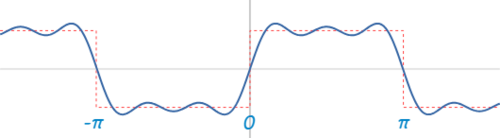
Answer: The link in the image on the left was clear enough as a good introduction, and I won't repeat it. The more interesting story about vectors in relation to those series is then.

1. In short, a Fourier series is the expansion of a periodic function into a sum of trigonometric functions. Since these functions form a vector space, there are (infinite) bases of orthogonal "vectors" with which they can be represent-ed. They are abstract vector spaces whose elements, i.e., vectors, satisfy the fo-ur basic axioms and therefore inherit their theorems, applications, and other consequences. One such orthonormal basis is the sequence of sines sin(nx), for n ∈ ℕ.

2. For example, one such basis is a sequence of sine functions sin(nx) each divided by √π along the interval from 0 to 2π. They are normalized:

\[ \frac{1}{\pi}\int_0^{2\pi} \sin^2(nx)\ dx = \frac{1}{\pi} \int_0^{2\pi} \frac{1 - \cos(2nx)}{2}\ dx = \] \[ = \frac{1}{2\pi}\int_0^{2\pi} \ dx - \frac{1}{2\pi}\int_0^{2\pi} \cos(2nx)\ dx \] \[ = \frac{1}{2\pi}x\Bigg|_0^{2\pi} - \frac{1}{2\pi}\frac{\sin(2nx)}{2n}\Bigg|_0^{2\pi} = 1, \]

because for every n ∈ {1, 2, 3, ...} this sine is zero. They are orthogonal:

\[ \frac{1}{2\pi}\int_0^{2\pi}\sin(kx) \sin(nx)\ dx = \] \[ = \frac{1}{2\pi} \int_0^{2\pi} \frac{\cos(k-n)x - \cos(k+n)x}{2}\ dx \] \[ = \frac{1}{2\pi}\left[\frac{\sin(k-n)x}{2(k-n)} - \frac{\sin(k+n)x}{2(k+n)}\right]_0^{2\pi} = 0, \]

when k ≠ ±n, because then these sines are zero.

It is further possible to write for (almost) every function f(x):

\[ f(x) = b_1\sin x + b_2 \sin 2x + b_3 \sin 3x + ... = \sum_{n=1}^\infty b_n \sin nx \]

and find the first few of these coefficients b_n which otherwise quickly tend to zero as the index n increases. With more summations the accuracy of the app-roximation f(x) becomes better.

3. Now it is easy to apply what was said above for sines analogously to cosines, finding that it is possible for (almost) every function f(x) to write:

\[ f(x) = a_0 + a_1\cos x + a_2 \cos 2x + a_3 \cos 3x + ... = \sum_{k=0}^\infty a_k \cos kx \]

and find the coefficients of a_k which also converge quickly.

4. Moreover, we also have a complex approximation, a sequence of orthonor-mal vectors e^inx, i² = -1, then divided by the constant √(2π), because:

\[ \frac{1}{2\pi}\langle e^{ikx} | e^{inx}\rangle = \frac{1}{2\pi}\int_0^{2\pi} e^{ikx}e^{-inx}\ dx = \] \[ = \frac{1}{2\pi}\int_0^{2\pi} e^{i(k-n)x}\ dx = \frac{1}{2\pi} \int_0^{2\pi} 1\ dx = 1, \quad k = n, \] \[ \frac{1}{2\pi}\langle e^{ikx} | e^{inx}\rangle = 0, \quad k \ne n. \]

This is already the third way of expanding the same function into a Fourier series with a series of new coefficients, say the notation c_n.

5. These are not the only ways to represent periodic functions using pieces of other functions, nor do they have to be periodic (when we look at part of the domain), but we can pause here and notice, for example, the free particles of quantum mechanics. They have these (4) exponential forms in their wave fu-nction notation.

In other words, we write arbitrary functions as sums of infinitely many free wave-particles, not all of which are necessarily real. In this way, we also understand them as sums of information. So, in addition to the remark that there are no shapes of the smallest particles (Volume II), the expansions of functions by Fourier and similar methods are actually a confirmation of my theories.

Solving » srb

Question: Can you give me an example of the Fourier series expansion of a function?

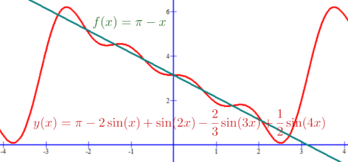
Answer: The figure on the right is the graph of the function:

f(x) = π - x.

That green descending straight line penetrates the abscissa and ordina-te at points π. Fourier transform:

\[ f(x) = \pi + \sum_{k=1}^\infty \frac{2(-1)^k}{k}\sin(kx), \]

has only k = 1, 2, 3, 4. That slice of the sum is an arced graph y(x) of red color with Fourier approximation on the abscissa interval from -L = -π to L = π.

1. We are looking for a duplicate of the function f(x) = π - x, for -L ≤ x ≤ L, in the form:

\[ f(x) = \sum_{k=0}^\infty a_k \cos\frac{k\pi x}{L} + \sum_{n=1}^\infty b_n\sin\frac{k\pi x}{L} \]

and, finally, we will take L = π, but first, let's know the common places.

2. Check the orthogonality:

\[ \int_{-L}^L \cos\frac{k\pi x}{L} \cos\frac{n\pi x}{L}\ dx = \begin{cases} 2L, & k = n = 0, \\ L, & k = n \ne 0, \\ 0, & k \ne n, \end{cases} \] \[ \int_{-L}^L \sin\frac{k\pi x}{L} \sin\frac{n\pi x}{L}\ dx = \begin{cases} L, & k = n, \\ 0, & k \ne n, \end{cases} \] \[ \int_{-L}^L \sin\frac{k\pi x}{L} \cos\frac{n\pi x}{L}\ dx = 0. \]

Use the trigonometric formulas product into sum, and sin kπ = 0 for all k ∈ ℤ.

3. Multiply both sides of equation (1) by cosine and integrate:

\[ \int_{-L}^L f(x)\cos\frac{m\pi x}{L}\ dx = \] \[ = \int_{-L}^L\left( \sum_{k=0}^\infty a_k \cos\frac{k\pi x}{L} + \sum_{k=1}^\infty b_k\sin\frac{k\pi x}{L}\right) \cos\frac{m\pi x}{L}\ dx \] \[ = \sum_{k=0}^\infty a_k \int_{-L}^L \cos\frac{k\pi x}{L} \cos\frac{m\pi x}{L} \ dx + \sum_{k=1}^\infty b_k \int_{-L}^L \sin\frac{k\pi x}{L} \cos\frac{m\pi x}{L} \ dx, \] \[ a_0 = \frac{1}{2L} \int_{-L}^L f(x)\ dx, \quad a_m = \frac{1}{L} \int_{-L}^L f(x) \cos\frac{m\pi x}{L}\ dx, \]

for m = 1, 2, 3, ...

4. Then, we multiply both sides of (1) by the sine and integrate:

\[ \int_{-L}^L f(x)\sin\frac{m\pi x}{L}\ dx = \] \[ = \int_{-L}^L\left( \sum_{k=0}^\infty a_k \cos\frac{k\pi x}{L} + \sum_{k=1}^\infty b_k\sin\frac{k\pi x}{L}\right) \sin\frac{m\pi x}{L}\ dx, \] \[ b_m = \frac{1}{L} \int_{-L}^L f(x) \sin\frac{m\pi x}{L}\ dx, \quad m = 1, 2, 3, ... \]

and that's it. Let's apply this to our problem, where f(x) = π - x and L = π.

5. We calculate the Fourier coefficients (3) and (4):

\[ a_0 = \frac{1}{2L} \int_{-L}^L f(x)\ dx = \frac{1}{2\pi} \int_{-\pi}^{\pi} (\pi - x)\ dx = \pi, \] \[ a_k = \frac{1}{L} \int_{-L}^L f(x)\cos\frac{k\pi x}{L}\ dx = \frac{1}{\pi}\int_{-\pi}^{\pi} (\pi - x) \cos(kx)\ dx = 0, \]

because for every k = 1, 2, 3, ... this integral is zero. Then:

\[ b_n = \frac{1}{L} \int_{-L}^L f(x) \sin\frac{n\pi x}{L}\ dx = \frac{1}{\pi}\int_{-\pi}^{\pi} = \frac{1}{\pi} \int_{-\pi}^{\pi} (\pi - x) \sin(nx)\ dx, \]

b_n = 2(-1)ⁿ/n,     n = 1, 2, 3, ...

6. We substitute these specific values ​​(5) into equation (1) and get:

\[ f(x) = \pi + \sum_{k=1}^\infty \frac{2(-1)^k}{k}\sin(kx), \]

and that is the Fourier transform listed next to the graph above.

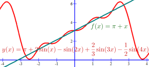
7. The image on the left shows another example, the function:

f(x) = π + x,

done in the same way. Now the ori-ginal graph is the increasing green line, and the winding red curve is the Fourier transform. This appro-ximation is for the practice, and the image shows the four terms of the sum:

\[ f(x) = \pi - \sum_{k=1}^\infty \frac{2(-1)^k}{k}\sin(kx). \]

Move on to more complex functions later.

8. A linear combination of functions corresponds to the same combination of their Fourier approximations. We know that different observers at the micro level will perceive the same reality differently, and now we see the reason, the logical consistency of these phenomena. Nature, deep in the foundations of its own mathematics, hides the possibility, or rather the sustainability, of unique-ness of subjects.

Importance » srb

Question: The meaning of dimensions in the Fourier series expansion of a fun-ction is strange, isn't it?

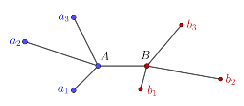
Answer: Yes, unless you are an ex-pert in the achievements of linear algebra. However, such a "strange" connection of functions with dime-nsions can be understood in other ways. I will try to explain some of it.

1. For example, graph theory will see the image on the right as, say, equal connections of small nodes a_i with large A, small b_j with large B (i, j = 1, 2, 3), as well as A—B, the connection of large ones. Someone will understand these connections as acquaintances of people, where only rare ones (A and B, unlike a_i and b_j) have large acquaintances; an economist could imagine equal flows of money and "strange" reasons for separating the few large ones from the many small ones. That such wonders really exist is also evidenced by sto-ries about six degrees of separation.

My information theory sees this as the principle of minimalism. Connections are the paths of communication, through the senses, or the ways of interaction that flow between the smallest in the world of physics in equal packets, quanta of action, which tend to inaction, or at least not to ripple, their status quo. Th-at is why the free market for money, goods, and services self-organizes towa-rds a network with fewer "degrees of separation." They are more fluid, more efficient, and more parsimonious "communications" (read: mediations).

2. Shannon (1948) could see in that graph a greater representation of some le-tters of the alphabet, which would make it less descriptive in words containing them compared to rare letters. For example, when we know in Serbian that the search term contains the rare letter "dž," this is important information becau-se it directs us to a narrow choice: jumbo jet, jam, chimney, and similar rare ones, unlike, say, the information that the name of the country in question co-ntains the letter "a," as almost every country has that letter in its name.

Then the nodes of the network with large A and B are less informative than the small nodes a_i or b_j. In my theory of information, we say that large attracts be-cause nature tends to states of less information, i.e., greater probability or less action. Larger nodes are crossings. They are the basis for gluing the natural phenomena, which we therefore recognize as natural laws. For the same reas-on, our brain prefers the familiar, and we consider creativity exceptional. It is this minimalism that lies deep in the foundations of inertia as a general natu-ral phenomenon, but also of our laziness.

3. We will recognize this "laziness" of communication in the work of artificial intelligence in its efficiency, or we already see it in existing social networks in the closure of our circle of "friends" into balloons of like-minded people and searches that are more frequent for us. This is how we come to the "dimensi-ons" of the above question.

If we remove the large node A from the communication of the above network, we will also remove the connection B with the small nodes a_i. We also see how a large frequency (of a large A) contributes to an increase in the frequency of each of its attached (small a_i), but also the concept of the basis of a vector spa-ce. Adding a new vector to the basis, independent of the previous ones, incre-ases the dimension of that space by including all the vectors connected to it.

4. Therefore, a coordinate system is a graph with points, nodes that are con-nected by their coordinates to each of the dimensions. Consistent with the principle of minimalism, it is an inefficient graph of communication, and, in accordance with natural tendencies, nature does not organize space as we define it in geometry.

Physical movements are limited by the speed of light, c ≈ 300,000 km/s, and this also applies to information. Thus, the present is a small island from which messages from the past arrive, and, in fact, they establish the situation of the aforementioned graphs with nodes in the present and their pasts, which have fewer and fewer connections, that is, have fewer and fewer communications with the rest of the universe. The more distant past is in the situation like the more distant terms, the coefficients of the sin(nx) in the Fourier expansion of the given function, relative to the given present.

Periodicity II » srb

Question: Why are there so many periodic natural phenomena?

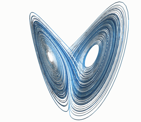
Answer: Periodicity is primarily cl-ose to reality which is observable, permanent, and true. The require-ments of permanence, in fact the laws of conservation like the more widely known ones for energy, ma-ke real phenomena finitely divisible (Packages), and then not more nu-merous than countable infinity. The periodic repetition of the state then comes by necessity, as with decima-ls of rational numbers.

However, the present is not all of reality. It is nuanced with the ways of perception by its unique subjects; it is dynamic, woven of uncertainty, and therefore constantly escapes from complete Periodicity. By advancing in (qu-antum) portions, it must leave the door ajar to other infinities, which are also, in their abstract way, perceptible. There is no contradiction, because we can-not reach infinity and it is not for us (the subjects of reality) to see an end to changes.

1. We make a recursion: add the number a = 1 to the number x, multiply by the number b = 3 and, if it is divisible, divide by the number c = 2. For exam-ple, we get the sequence:

10, 33, 16, 51, 25, ..., 7, 24, 12, 6, 3, 6, 3, ...,

and after 16 steps the triplet 12, 6, 3 is constantly repeated. The another exa-mple, a = 1, b = 3 and c = 2 generates an infinitely growing sequence:

1, 4, 10, 22, 46, 94, 190, 382, ...

in which there is no repetition of numbers. The difference between the first and second examples is that the value of the first is returned and, due to the finite number of possibilities up to some maximum, the value of some incide-ntal x is repeated, and so the further sequence that follows it is repeated. Such a loop is avoided in the unlimited increase of the current number x in the sec-ond example.

2. A similar pattern is found in opening links on the Internet, which will alw-ays end in a loop if the number of pages is finite and static. When there are a large number of places to call, we may not notice the periodicity of the proce-ss, but if the number of sites is very large and their evolution is noticeable, th-en the absence of periodicity can occur despite the constant finiteness of the possibilities.

I explain the resolution of the seemingly paradoxical atomization of phenom-ena and processes due to finite divisibility, and this is due to the duration of reality (a property of infinity is the ability to be equal to its part) and, in con-trast, the fundamental uncertainty due to which the exact repetition of anyt-hing is not possible.

3. It is in the nature of "duration" to maintain quantity rather than essence, because the latter is more easily changed. Both change with their probabilities, which are more visible in the second case. Thus, a microparticle can appear multiple times or not appear at all and violate the law of conservation, but on-ly at such short intervals that its instability in the macro world is impercepti-ble. On the other hand, there are appearances of its other forms, or decays.

We are talking about the limitations of "reality" that make it analogous to mo-dels (1) that make it behave periodically, or almost periodically. When we di-vide the entire universe into "portions of positions" (small open neighborho-ods of points), it does not matter that there may be a continuum of free posi-tions (cardinality labels 𝔠), the added portions will be at most countably infi-nitely many (ℵ₀). Therefore, the periodicity of some states and phenomena is certain.

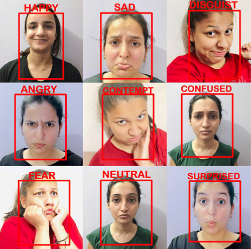
4. This is where the need for calculating similarity arises, for example, in bu-ilding artificial intelligence. Computer representations of faces are arrays of pixels in numbers that define position, tonality, and color, which we can easily treat as polygon angles and, say, find a significant "amount of similarity" with "smile" for the basic assumption "this face is smiling." There are two ways to measure the "amount of similarity" for further inference from others.

I personally developed methods for measuring the "amount of similarity" mo-re for testing in my game theory. When we find ways to convert situations on the field of a complex game into "pixels" (strings of numbers), then there is a need to compare such situations with each other, with similar ones, or with "good" or "bad" patterns in order to search for appropriate moves or reactions to the actions of the opponent (Reciprocity). Repetitions in player behavior are a great help to the programmer if he knows how to recognize and use them.

Sierpiński » srb

Question: I don't understand why infinite divisibility would violate the conser-vation law?

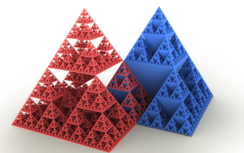
Answer: The link in the image on the right leads to the paradoxical Sierpinski triangle. It is a recursive separation of triangles from a tria-ngle so that in the end there remai-ns a "triangle" of area zero with in-finite perimeter. The same is achie-ved with other flat geometric figur-es or with geometric solids, for exa-mple, with the pyramids in the ima-ge on the right; their volumes tend to zero when cut, and the areas remain equal to the initial pyramid.

1. The following figure illustrates the scheme for adding edges to a Sierpiński triangle. Equilateral triangles are added to equilateral triangles, and their in-teriors are removed, in an infinite sequence.

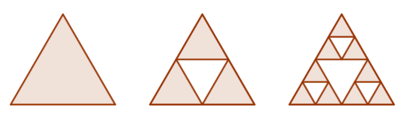
After each iteration, 3/4 of the area remains from the previous one. After the nth iteration, the remaining area is (3/4)^n-1 of the initial area, and this num-ber tends to zero as n grows indefinitely. However, in the nth iteration, we have 3ⁿ edges, each of which is half the length of the previous one, it is 2^-(n-1) the length of a single edge of the initial triangle. Therefore, the length of the edges of the nth iteration is:

\[ 3^n\cdot \frac{1}{2^{n-1}} = 3\cdot\left(\frac32\right)^{n-1} \to 0, \quad n \to \infty. \]

So the area of ​​the Sierpiński triangle tends to zero as its edge lengths increase infinitely. You can do the same with many shapes.

2. To avoid referring to the definition of infinity (a quantity that is equal to its proper part), which is probably confusing, as in the question I was asked, I will refer to the principle of minimalism. Nature spontaneously tends to states of smaller emissions of information, higher probabilities, and smaller actions. In the case of infinite division, when infinite lengths arise in relation to negligible areas or unlimited areas of figures in parallel with their limited volumes, then (in my theory) infinite emissions of information occur. And that is the impos-sible mission, because lengths and areas are equivalent to information, and their emissions are so large that they are unnatural.

3. We can also look at it this way. In thinking about the example (Periodicity II, 1), one can also encounter recursion; for example, adding a = 15 to the cu-rrent number x, and then multiplying them by b = 2, unless the number x is divisible by c = 12 and is thus divided. Namely, if the start number x = 3⋅12^k, for k = 0, 1, 2, 3, ... one reaches the repetition 36, 3, 36, 3, 36, 3, ... but for each starting x ≠ 3⋅12^k an unlimited increase in the current x occurs. This requires (discretely increasing) jumps to avoid infinities.

For example, when the initial x₁ = 3, then the following is true:

x₂ = (x₁ + a)⋅b = (3 + 15)⋅2 = 36,

and this is divisible by c = 12, so x₃ = 3 and the process is repeated. However, when x₁ = 4, 5, 6, ... divergent sequences arise:

4, 38, 106, 242, 514, 1058, 2146, 4322, 8674, 17378, ...,
5, 40, 110, 250, 530, 1090, 2210, 4450, 8930, 17890, ...,
6, 42, 114, 258, 546, 1122, 2274, 4578, 9186, 18402, ...

However, for x₁ = 3⋅12², 3⋅12³, 3⋅12⁴, ... we obtain periodic sequences:

432, 36, 3, 36, 3, 36, 3, 36, 3, 36, ...,
5184, 432, 36, 3, 36, 3, 36, 3, 36, 3, ...,
62208, 5184, 432, 36, 3, 36, 3, 36, 3, 36, ...,

which are like lonely islands in a sea of ​​singular points around them.

4. Similar restrictions, but with fewer singularities, exist for the Fourier transform, say on the interval x ∈ [0, L] and with complex coefficients:

\[ c_n = \frac{1}{L} \int_0^L f(x)e^{-inx}\ dx, \quad n \in \mathbb{Z}, \]

with which the approximation of the function (Fourier) will be valid, when in a given interval there are no singular points, places with infinite values ​​of the function f(x) to be replaced.

For example, more precisely, the Fourier series of the function f(x) will conve-rge absolutely (therefore uniformly), if f satisfies the Hölder condition of order α, with α > 1/2, i.e.

\[ \sup_\theta |f(\theta + x) - f(\theta)| \le A|x|^{\alpha}, \quad \forall x. \]

This condition cannot be met with a singularity of a function that would make infinite jumps.

5. Mathematics allows for consistent substitution, such as the exchange of po-sitions (states x = ωt) with processes (t), which physics might be able to inter-pret someday, if ever. However, problems with singularities in mathematics will almost always be problems of interpretation, and that is why we empha-size them. Here, in particular, Fourier series approximations easily lead to information representation, and the aforementioned Hölder condition beco-mes indispensable. We now see it as the reason for the discreteness (quanti-zation) of physical information.

I mean, we don't know what the particle-waves, or probability waves of quant-um mechanics, "approximate" when we say they are the result of Fourier tran-sforms. We can equally assume that the intervals below are full of all sorts of singularities of some functions that we have no idea what they are, and that in the end it doesn't matter. Simply put, nature packages its wonders in such a way that for us, its subjects, there is no real answer to the question of what is cooked in them and who the cooks are.

Logarithm » srb

Question: What is the role of logarithms in your information theory?

Answer: The Logarithm is still im-portant in measuring the "amount of possibilities", but not as much as it once was. A good example is bi-nary search.

1. Let's say we are looking for the number 3 in the sequence from 1 to 8. The first dilemma is to choose half, its subsequence 1, 2, 3, 4. The second is to find half of that half 3, 4. In the third, the desired number is 3. Without going into methods, such as the questions that start with "does..." attached in the link, we have the "quantity of possibilities" log₂x = 3 among x = 8 candidates. It is this logarithm of Hartley (1928) that was the inspiration for Shannon (1948) to develop the now largely classical theory of information.

Namely, there is no information without uncertainty, and this requires at least two possibilities 0 and 1, and that dilemma carries the information value 1. When we have a "dilemma of dilemmas", there are already four possibilities 00, 01, 10 and 11, or 2² = 4 and information 2. This is a matter of combinato-rics (a branch of mathematics), so much so that the composition of "three dilemmas", as we know in advance, has 2³ = 8 possibilities:

000, 001, 010, 011, 100, 101, 110, 111

and the information valued 3. In general, h = 2^m, with h Hartley information and m number of equally likely possibilities. Inversely, m = log₂h and we are still familiar with the logarithm story.

2. When there are m equally likely options, the probability of one is p = 1/m. And since nature doesn't like equalities, we round up. So, when something happens on average once in five attempts, we say that its probability is p = 1/5. We make sense of that, and we assign an outcome with probability 1/5 to an event with 5 equally likely possibilities, even though none of them are there. That's just one way to understand Hartley's information, the logarithm:

h = log₂ m = -log₂(1/m) = -log₂ p,

as information of an arbitrary probability p ∈ (0, 1). The mean value of the information of the probability distribution is (p₁ + p₂ + p₃ + ... = 1, ∀p_k > 0):

S = -p₁⋅log₂ p₁ - p₂⋅log₂ p₂ - p₃⋅log₂ p₃ - ...,

and that's Shannon information. Again logarithms, but also approximations. I used the next one (Nearli), but I don't know if it ever caught on anywhere.

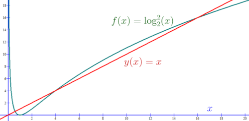
3. When a distribution has infinitely many outcomes, then only finitely many of them have probability one (Borel-Kantelli lemma). Hence it makes sense to round up, work with significant samples instead of all, or again use the appro-ximation (log₂m)² ≈ m, for values ​​of m ∈ (2, 20). It can be seen in the graph on the left, and m is then the predominant number of possibilities. Shannon's information thus becomes:

\[ S \approx \frac{1}{\sqrt{m_1}} + \frac{1}{\sqrt{m_2}} + \frac{1}{\sqrt{m_3}} + ... \]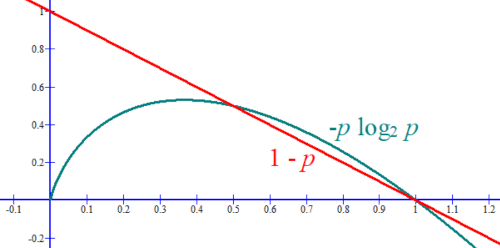

For higher probabilities p ∈ (1/2, 1), the approximation p⋅log₂ p ≈ 1 - p. It is sketched by the graph on the right. Some other approximations are possible, and I use them only in cases that cry out for simplified de-scriptions. They help to understand the generalization and to bring the interlocutor closer to something th-at becomes obvious to them over time, that many expressions of quantum me-chanics are not far from information. And on the other hand, when p → 0, th-en p⋅log₂ p → 0, as can be seen in the same figure on the right. Hence, we can ignore Shannon summands of low probability.

4. For example:

\[ \frac13 + \frac14 + \frac15 + \frac16 + \frac{1}{20} = 1 \] \[ -\frac13\cdot\log_2\frac13 - \frac14\cdot\log_2\frac14 - \frac15\cdot\log_2\frac15 - \frac16\cdot\log_2\frac16 - \frac{1}{20}\cdot\log_2\frac{1}{20} \approx 2.140 \] \[ \frac{1}{\sqrt{3}} + \frac{1}{\sqrt{4}} + \frac{1}{\sqrt{5}} + \frac{1}{\sqrt{6}} + \frac{1}{\sqrt{20}} \approx 2.156 \]

rounded to three decimal places. These probabilities do not have to be the Egyptian fractions; it is enough that they are of similar values.

5. A slightly more general expression for the wave function of a free particle is:

\[ \psi(\mathbf{r}, t) = Ae^{i(\mathbf{p}\cdot\mathbf{r} - Et)/\hbar}, \]

where A is a constant, p = (p_x, p_x, p_x) is the momentum vector, r = (x, y, z) is the position vector, E is the energy, t is the time of the particle, and ℏ = h/2π is the reduced Planck's constant, with an imaginary unit (i² = -1). The values ​​of the exponents are very small and their imaginary part in the macro world is negligible. However, we can recognize a series of orthogonal vectors:

\[ \psi_k(\mathbf{r},t) = e^{ik\varphi t}, \quad \varphi = (\mathbf{p}\cdot \mathbf{v} - E)/\hbar, \quad k \in \mathbb{Z}, \]

as a basis of a vector space in which the above wave function is a special case of a linear combination:

Ψ(r, t) = ∑_k A_k ψ_k(r, t),

with a series of constants A_k. Also, it is a Fourier expansion. To all this, one can add the expansion of these concepts to ψ as the number of possibilities, and φ with or without factors in the exponent, as information. Again, we have information φ as the logarithm of the possibility ψ, but then as a complex logarithm, which is a periodic function, which is how we represent particle-waves.

Facial » srb

Question: What vectors do you use for facial expression recognition?

Answer: I've actually used vectors in game simulations and other tests of my theories and never in practi-ce, except to spread some of these ideas in correspondence, and then who knows what others might have used them for. That's the trouble with theory: everyone is, which is opposed to the concrete, which is unique.

The nice thing is that such a model is easily transferable to reading fa-cial expressions. The idea is the amount of similarity which I have already presented in several answ-ers. It is no longer a secret that the similarity of n-th angles is not measured by the direct difference of the angles, but by the determinant of the matrix that maps one to the other. All triangles have a sum of angles of 180°, so we normalize everything we compare to that value. Then the lengths of the sides no longer matter, that is, it does not mat-ter whether the head is large, or the person is far away, or even whether he is wearing a mask in some cases. And the value of that determinant is easily de-termined without finding the determinant itself.

To make it short, a digital image is in pixels that are recorded by a series of numbers, and they also contain color data (Triads II). When you only want the shades of that color (RGB), you sort them and then normalize by the number of components of the series (vectors) as well as by their sum — according to the patterns of expressions that should be on the side in the database. From the mapping of the vector (image) from the terrain to the database vector, the one with the maximum determinant is taken, and, for example, if there was a "smile" in the database, with a sufficiently high value of the determinant, the conclusion is "this face is smiling." All the other stages described here are routine today, except for this determinant method, which, I believe, is a novelty.

In the case of a game, weighing the actions of opponents who strive for victo-ries, when we have a "good" move of the opponent for the home player scored with positive numbers and a "bad" one scored with negative values, we also use pseudo-stochastic matrices (Stochastic II). I sought the main success of the described method of determinants and, I hope, found it in its agreement with the previously used method of scalar multiplication (Win Lose), or sum of products, i.e. information perceptions. This older one is based on the amo-unt of vitality as a measure of the strength of the game.

Consent » srb

Question: Can you explain to me the "agreement" between measuring similari-ty using the determinant method and the sum of products?

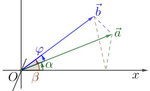
Answer: The figure on the right sh-ows a sketch of the arrays, vectors: a = (a₁, ..., a_n) and b = (b₁, ..., b_n) in some n-dimensional rectangular coordinate system. Also the angles ∠(x,a) = α and ∠(x,b) = β abscissas to the first and second, and angle ∠(a, b) = φ between the first and second. These are sorted arrays of the angles of two n-th angles, say, the largest component to the x-axis.

1. This means that tripod xab has the least of such angles of the given vectors and that is almost φ = β - α, if β > α. In other words, when the determinant of the matrix A : a → b which maps the angles (Similarity II) showed a larger va-lue, then the scalar product a⋅b = |a||b|cos(φ) is also larger. Since det(A) ≤ 1, it is practical to normalize these vectors to unit length using the 1-norm (the sum of the absolute values ​​of the components), because their component sums are already equal (these are the sums of the nth angles polygon).

The determinant we are talking about is special, from a specially chosen matr-ix and the value is the product of diagonal elements that are different from 1 of each k-th component when a_k > b_k and which is d_k = b_k/a_k. So, we have the determinant det(A) = d_k d_k' d_k'' ..., and on the other hand the scalar product a⋅b = a₁ b₁ + a₂ b₂ + ... = |a||b|cos(φ). When the first value increases, the se-cond also increases and vice versa.

2. Let's look at this in one of the first examples (Similarity, 2), but with vectors (Ax₁ = x₂) divided by 180° for normalization in the Manhattan norm:

\[ \begin{pmatrix} 1 & 1/12 & 1/6 \\ 0 & 11/12 & 0 \\ 0 & 0 & 5/6 \end{pmatrix} \begin{pmatrix} 1/2 \\ 1/3 \\ 1/6 \end{pmatrix} = \begin{pmatrix} 5/9 \\ 11/36 \\ 5/36 \end{pmatrix}, \quad \det(A) = \frac{11}{12}\frac56 \approx 0.764. \]

3. This norm, L₁, is greater than L₂ (the Euclidean norm), for example:

∥x₁∥₁ = |1/2| + |1/3| + |1/6| = 1,

∥x₁∥₂ = (|1/2|² + |1/3|² + |1/6|²)^1/2 ≈ 0.624.

However, in the Euclidean norm we express the scalar product, so it is:

x₁⋅x₂ = α₁α₂ + β₁β₂ + γ₁γ₂ =

\[ = \frac36\frac{20}{36} + \frac26\frac{11}{36} + \frac16\frac{5}{36} = \frac{87}{216} \approx 0.403. \]

4. It happens that the results of the scalar multiplication x₁⋅x₂ are smaller than the determinant of the mapping A : x₁ → x₂, but we will not confuse this with the previous statement because det(A) and x₁⋅x₂ are not metrics. Here it is en-ough for us that they agree. If we need metrics, say L₁ and L₂, then we find in order:

d₁(x₁, x₂) = |α₁ - α₂| + |β₁ - β₂| + |γ₁ - γ₂| ≈ 0,111

d₂(x₁, x₂) = (|α₁ - α₂|² + |β₁ - β₂|² + |γ₁ - γ₂|²)^1/2 ≈ 0.068

rounded to three decimal places. They are also useful for comparing "amounts of similarity" in some circumstances.

Аnnulment » srb

Question: How is isometry even possible, if nature is forced to constantly change?

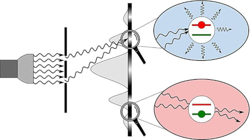
Answer: Isometry, an identical ma-pping, does not change the distan-ces between points; that is, it does not affect phenomena that can be reduced to distances. However, my theory of information says everythi-ng is news, and that as soon as it is communicated, it becomes stale and is no longer news. In addition, there is the law of conservation, which tells us how closed systems of aggregate quantities of uncertainty sur-vive. So the question posed makes sense.

1. From the point of view of the previously described "amounts of similarity" det(A), where A is linear mapping A : x₁ → x₂ of the vector x_i = (ξ_i1, ξ_i2, ..., ξ_in), the question arises about the meaning of isometry in a special way. The men-tioned determinant is maximal (one) when its columns, as vectors, span the largest volume. Thus, the largest (complete) similarities give such comprehe-nsive mappings that do not leave even the slightest gaps in the space with wh-ich they form new images. But when an identical copy is truly impossible, then we get by by coming up with a more realistic scenario.

For example, like the dark state of atoms or molecules from which they cannot emit energy. With newer quantum physics, these are becoming less hypotheti-cal, as can be seen in the text accompanying the image above left. In my theo-ry, they are examples of extinguishing the original information after its emiss-ion (the reported news is no longer news) by the aforementioned optimal cou-rse of events A forming a maximum copy, the most it can do is completely nul-lify what it acts on, which could, like the phoenix regenerate again.

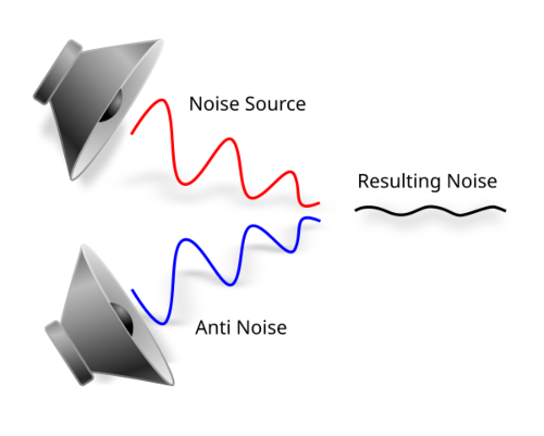
2. Sound-blocking technologies ha-ve long existed. Large rocket launch sites have sound-blocking systems to absorb or deflect the acoustic en-ergy of a rocket launch, and more recently, headphones for everyday use have similar methods.

The sound that reaches the ear is recorded and reproduced with a phase shift so that the interference cancels out the incoming sound. Algebraically, we have a described isometry of noise that leaves a copy in almost the same place, that is, at a close moment. And the same thing happ-ens in order for something different to happen, to put it simply.

3. A wave in motion, undisturbed by other actions, changes its isometries in at least two steps. A similar example is the minimal polynomial of a matrix. This follows from the property of a matrix of order n to span space at most n-dim such that the sequence of its degrees A⁰ = I, A, A², A³, ..., Aⁿ has at most n li-nearly independent terms. We write the eigenvalue equation Av = λv firstly as (A - λI)v = 0, and we see that the eigenvector v is from the null-space of the matrix A - λI. Since it is not regular, det(A - λI) = 0, and λ is one of the seque-nces λ₁, λ₂, ..., λ_n of the roots of that equation, i.e., the eigenvalues ​​of the matrix A.

Hence, the minimal polynomial of the matrix A is:

p(A) = (A - λ₁I)(A - λ₂I)...(A - λ_nI),

p(A) = Aⁿ + α₁A^n-1 + ... + λ_n-2A² + λ_n-1A + α_nI

and because p(A) = 0, say, Aⁿ is a linear combination of the lower n powers of this matrix. In this sense, as an n-term engine, every matrix is ​​like an n-term "isometry". For example:

\[ \begin{pmatrix} 1 & 2i \\ -2i & 3 \end{pmatrix}^2 - 4\begin{pmatrix} 2 & 2i \\ -2i & 3 \end{pmatrix} - \begin{pmatrix} 1 & 0 \\ 0 & 1 \end{pmatrix} = 0 \]

is the minimal polynomial of the matrix (A is in the middle), which is easy to check by exponentiation and addition. Therefore, the process in steps A, A², A³, ... can be considered "two-stroke" in the way that the same processes A and I always alternate, but constantly in new forms αA + βI with different constants α and β.

4. The universe is in constant recreation, rearranging its states and processes so that it is always new, so that no two of its states are repeated, because that is how things are in principle in this information theory. Therefore, all its par-ts are always different in relation to the whole. I have explained many times how this happens through the duration (of reality) and the deposition of the past, which increasingly affects the present less and less, and from which fo-llows the increase in current certainty from the decrease in the density of un-certainty, and then the increase in visible space. Another question is whether there are any real creations in this development.

Initiator » srb

Question: How does the force act? Is the force represented by force fields, su-ch as electromagnetic fields, or as is seen in Feynman diagrams with gauge bo-sons, or is it instead a property of the geometry of space similar to Einstein's gravity?

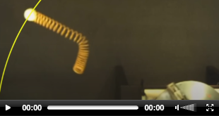
Answer: I believe that information underlies physical phenomena, and that concept cannot exist without change, time, and process. Physical forces are the consequences of the transfer of influence, not through “forces” or “pushing,” nor is space completely static as you describe. Force is the transfer of disturban-ces, in accordance with the princi-ple of minimalism, the more frequent occurrence of more likely outcomes, or differences in action. They move the environment at the speed of light, which we see stopped in the time in which we flow.

1. If the Sun suddenly disappeared, the Earth would continue to move in its orbit for the next 8.3 minutes, which is the time it takes for information from the past to tell it. Stars also explode or collide, and sudden changes in their behavior are not impossible. We also know of other gradual changes in the influence of the force, such as the one described in the video image above left.

A spring that is at rest hanging alone or holding a ball, when suddenly releas-ed will contract from top to bottom and the lower end will remain at rest until the center of mass reaches the bottom of the spring sandwiched between its lower and upper ends. This seems absurd when we only observe the weight (ball) at the bottom which during this contraction is at rest, does not sink but floats as if it does not feel gravity. This also happens in circular motion with a ball on a spring that, unhooked, goes in a circle as the center of mass approa-ches its end.

2. These were unusual situations of the known laws of physics since the time of Newton (1687) so that we might understand our confusion more easily. Processes are defined by the states they act on and the states of the processes themselves. But one can also speak of zero changes, so bodies move along conic sections under the action of a central force even if that force is zero, because a straight line is also a conic (Orbits II).

In this sense, space is a storehouse of information whose manifestation is resisted by the principle of minimalism, probability forces, which are in equilibrium when we consider that there are no external actions. Therefore, in space outside of forces, there are actually uniform tensions here and there, whose processes we measure as zero and say that they do not exist. Moreover, we can speak of any (zero) flow of space due to which a body in a weightless state is at rest, like a ball hanging on the end of a spring that has just been released.

3. That this idea is not empty can be seen from, say, observing a hanging spr-ing and its release, so that the upper end will begin to approach the lower one while the lower one remains at rest, regardless of altitude, that is, in an incre-asingly weaker gravitational field until zero. It will happen that at high altitu-des, in a weaker gravitational field, the spring will be less stretched and the contraction process will be less dramatic. We do not ignore all such things until finally zero. It is similar with a spring attached at various lengths that rotate at the same or different angular speeds.

Similar to this is the emission of virtual photons from electrons that either be-come real by interacting with another electric charge, or do not exist if their interaction does not occur. There is no repulsion (attraction) without inform-ation exchange, which can also explain the "Schrödinger's cat", the lack of an exact trajectory of the electron before measurement (Heisenberg). The que-stion in the title, according to this, ignores the constant tension that space itself has and the waiting for an opportunity for such tension to manifest. The presence of a visible force is the disturbance that initiates this manifestation.

4. It is possible that each of the ideas in the question is valid. Such are correct theories, they are multi-valued. The number π = 3.14..., for example, can be found from geometry as the ratio of the circumference and diameter of a circle, or by solving the Basel problem, or by probability theory (Buffon's needle). Each time equally correct, but in a different interpretation. Moreover, none of these will be a definitive, readable book without possible sequels. Therefore, these questions can equally make sense, as can overcoming their meaning.

Dzhanibekov » srb

Question: Can you explain the Dzhanibekov effect to me again?

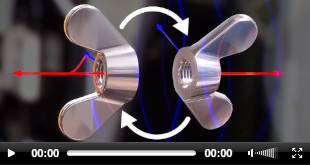
Answer: Watch the video on the ri-ght and then try to go a little furth-er. Throwing a tennis racket while catching it again by the handle, let's watch it inexorably rotate around its three axes: longitudinal, trans-verse and flat. This is what the in-termediate axis theorem says, and hopefuly I can talk about it a little differently.

1. Torque (Torque) is the force \(\vec{\tau} = \vec{r}\times \vec{F}\), which is the (Volume II) vector pr-oduct of the force that rotates the body and the vector of its shortest distance from the axis of rotation. It is the force that keeps the gyroscope always poin-ted in one direction, along the axis of its rotation, like a top. It is perpendicu-lar to the vectors \(\vec{r}\) and \(\vec{F}\), so it is perpendicular to the plane of rotation and is taken to have a right-hand rule direction. However, what if there is an additi-onal axis of rotation?

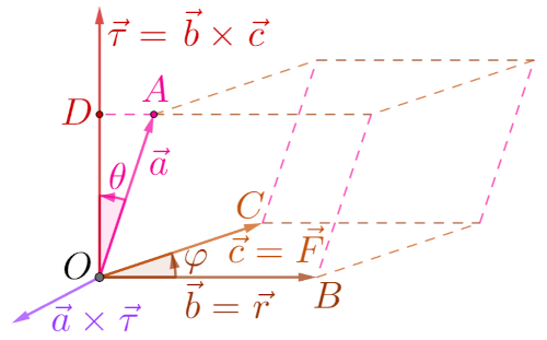
2. Let's look at the image from the beginning of this blog again and make a few changes to the left to prove the formula:

\[ \vec{a}\times (\vec{b}\times \vec{c}) = (\vec{a}\cdot\vec{c}) \vec{b} - (\vec{a}\cdot\vec{b}) \vec{c} \]

double vector product. The bracket on the left holds the vector \(\vec{\tau}\), the torque, so it is a vector perpendic-ular to both \(\vec{a}\) and \(\vec{\tau}\), that is, it lies in the plane of the vectors \(\vec{b}\) and \(\vec{c}\). Thus, we have established that the double vector product is a linear combination like the expression on the right.

It changes sign if the vectors \(\vec{b}\) and \(\vec{c}\) swap places, which means that the coef-ficient in front of the first one also changes with the minus coefficient in front of the second one in their linear combination. Since the coefficient in front of the second of these three vectors must be linear in the first and third, we fina-lly find that the formula is correct. You will find a detailed analytical proof in the book Quantum Mechanics (Vector triple product).

3. The plane OBC is crossed by the second and third vectors from the above equation and rotates around the vertical axis OD, so when the perturbation makes the first of these vectors, it will start to tumble, to rotate around the axis that extends through itself. This happens in the video above when turn-ing a bottle with liquid, so it is said that its kinetic energy is converted into heat. I hope you now have a more detailed explanation.

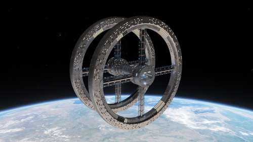
Huge space stations, like the one in the picture on the right, inspired by science fiction stories and movies today, which generate artificial gr-avity in rooms on the outer rim of rotation, could have this tumbling problem with their gyroscopes. Such problems could occur in all spacecraft that circle in ordinary orbits around the Earth.

4. In scientific works on the same topic, I am not sure that this "anomaly" of gyroscopes has been sufficiently noted. We see it with a twist as a circular os-cillation of the axis of their rotation. Hence, the axis of the Earth's daily rota-tion also wobbles due to the revolution around the Sun. Our mathematician Milutin Milanković took the phenomenon into account when he studied ice ages and in doing so found the most accurate calendar to date. At that time, he was not so much concerned with the mathematical cause itself as with astro-nomical facts.

Adaptation III » srb

Question: How exact are the vectors you are talking about?

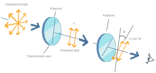
Answer: I understand you are ask-ing how accurate this theory (of in-formation) is, if it assumes the "ob-jectivity" of chance. The correct an-swer would be that I am not sure yet, although it is correct to act as if I am — until I eventually encounter at least some understandable contr-adiction.

I still find both versions of "information theory" logical and confusing, the first deterministic one that I started with and the second stochastic one that I find more developmental, so I'm giving it preference for now.

1. One of the reasons for the appeal of this second, stochastic version of infor-mation theory is its ability to adapt, not only the theory itself to circumstances but also its interpretation of nature as such, adaptable. For example, from the relations of uncertainty of the micro world to the great certainties of the big world (Accordance), the latter because of the laws of large numbers that make probability theory seem to encompass the first, deterministic version. And the former seems to exclude the latter.

The second type of “adaptability” in my contributions is already a classic, like the adaptation of a message to a channel as it passes through a series of links in a Markov chain. "You are what you are with" is a popular proverb, but here we should also think of all of nature, which adapts to its subjects proportiona-tely and much less to its individual participants than they do to its whole. Its dexterity in adaptation will also explain some coincidences.

2. An example of an adaptation that seems to be able to replace the objective uncertainty of quantum mechanics is Malus's law (link in the image on the left). It is the transmission of light through a polarizer whose intensity is the square of the amplitude, since the output is I = I₀ cos²θ, where I₀ is the inte-nsity of the incoming light and θ is the angle of inclination of the polarizer.

Namely, the light that passes through a vertical and then a horizontal polarizer will have an intensity I₀ cos² 90° = 0. However, when we separate these 90° into two polarizers of 45°, the result after the first is I₀ cos² 45° = I₀/2, which after the second gives I₀/4. We can say that the light in the first reset to new values, as it is said in the video Superposition Narrative, or simply adapted, th-us avoiding the probabilities from quantum mechanics that in their own way arrive at the same thing.

3. Adaptation is more natural to stochastic information theory, but it leads to illusions. If this and that can happen, then anything is possible and a bit ficti-onal. Thus, the states of light in polarization are, in general, similar vectors, just average values ​​with smaller or larger dispersions. They have their enviro-nment with some chances for something different, so if we give them a chance in small steps, they can manage to adapt, or in other words, to transfer that chance through the chain.

On the other hand, this chance has two faces, so the question is how "real" is something that could and could not be, to be with one that is not realized. Th-at there is no "reality" and that which is not realized, that is, that our "reality" consists to a significant extent of the unreal. In fact, therein lies the appeal of this stochastic theory of information, in its ability to penetrate life, to explain perhaps even the fantasies that drive physical reality.

4. To understand how natural this idea of ​​adaptation is, let us now take three polarizers, each tilted 30° relative to the previous one. Each transmits content cos² 30° = 3/4 of the light, so amount of these three is (3/4)³ = 27/64 ≈ 0.423 (42.3 percent) and is more than the previous two polarizers tilted 45° each, which transmit 1/4 = 0.25 (25 percent) of the light.

If we break the steps into small angles x → 0, then the transmittance of a si-ngle polarizer is cos²x and if there are 1/x at a right angle (we divide 90°, i.e. π/2 radians, into n = 1/x parts) the limit value is (cos²x)^1/x → 1. Namely, we put y = ln(cos x)^2/x, and then we apply L'Hôpital's rule:

\[ \lim_{x \to 0} y(x) = \lim_{x \to 0} \ln(\cos x)^{2/x} = \lim_{x \to 0} \frac{2\ln \cos x}{x} = -2\lim_{x \to 0} \tan(x) = 0, \]

so from y → 0, i.e. ln(cos x) → 0, it follows that cos x → 1. This means that the adaptation in these small steps is total, it transmits all the light intensity.

Divergence » srb

Question: Can space then be viewed as an adaptation to something?

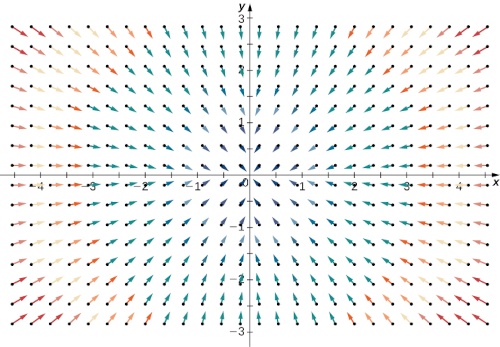
Answer: We discuss the previous topic, adaptation of light through a series of polarizers (Adaptation III, 4) and the possible extension of that idea.

Yes, I believe it is worth working on the "adaptation of space" and, say, some of Maxwell's equations (Information Coupling) as a type of such expressions. The founders of the theory of electricity and magne-tism, Ohm, Faraday, Gauss and others, could not have known about electrons, but they ingeniously successfully discovered their imprints in space and real consequences. According to the definition of reality (verifiability, maintaina-bility, truthfulness) that I only use here, they were on the right track.

1. In the image on the right we see the vectors of immersion into the origin of the plane Oxy. These are the vectors r(x, y) = (-x, -y) directed opposite to the coordinate axes. The divergence of that space, the field, is a constant negative:

\[ \text{div}(\mathbf{r}) = \frac{\partial}{\partial x}(-x) + \frac{\partial}{\partial y}(-y) = -2. \]

If these field vectors had opposite directions from the origin outward, it would be r = (x, y) and div(r) = 2. The divergence of a constant field, say at all points r = (2, 3), is zero, because the derivatives of the constants are zero. All partial derivatives of other, incorrect coordinates are also zero; hence a circular field, such as r = (-y, x), again has zero divergence.

Divergence is an operation on a vector field that tells us how the field behaves towards or away from a point. Locally, the divergence of a vector field F in ℝ² or ℝ³ at a particular point r(x, y) or r(x, y, z) is a measure of the "drain" of the vector field from that point.

If F represents the velocity of the fluid, then the divergence at point r measu-res the net rate of change with respect to time of the amount of fluid flowing out of that point (the property of the fluid to flow "out" of point r). Specifica-lly, if the amount of fluid entering point r is equal to the amount leaving, the divergence at that point is zero, hence the mentioned circular field is also of zero divergence. This is what we know well from the theory of electromagne-tics.

2. There are also examples of “space flow” in information theory, simply beca-use of its dynamic concept. Let’s not go too far now; let’s take the time dilation of the theory of relativity. It happens in the presence of masses, and then there are larger time flows in the surrounding space, compared to which the gravita-tionally denser parts lag behind in time. They mimic the arrows in the picture, all of which point towards the abyss and are longer the further away they are from it. This remains the case even when there is no connection with the ele-ctromagnetic field.

Whatever is coming from the future, the longer arrows are closer to it, but the bottleneck is around the abyss. There the outflow slows down, there is a delay in arrival. It flows more slowly because time flows more slowly. It opens up opportunities for theorists for various speculations. In other words, forces like the electromagnetic (Initiator) are still an open topic for research, not the ph-ysical forces themselves.

3. The future arrives everywhere at the same speed of light, c = 300,000 km/s, so let's assume that "something" of it can accumulate through differences in the flow of time. If it is a scalar quantity, it can be found as the scalar product of the vector flux density A(r) and the vector ds of the surface element S. Their total quantity F is the integral of the vector field:

\[ \int_S \mathbf{A}(\mathbf{r})\cdot d\mathbf{s} = F. \]

Here A is the flux density at point r. In particular, the flux of a vector field that would be of unit magnitude and normal to all points would be a surface.

The electric flux density D in units of C/m² will describe the electric field as an apparent density. The integral over a closed surface gives the total charge Q on the given surface, and this relationship is Gauss's law:

\[ \int_S \mathbf{D}(\mathbf{r})\cdot d\mathbf{s} = Q. \]

The magnetic flux density B in units of Wb/m² describes the magnetic field like a flux density. The integral over a surface (open or closed) gives the ma-gnetic flux Φ, which has units of Wb:

\[ \int_S \mathbf{B}(\mathbf{r})\cdot d\mathbf{s} = \Phi. \]

This formula is close to Faraday's law.

4. When we consider, say, a total charge Q in units C with a flux density D su-rrounded by a surface area S within some volume V, we can divide the above equation by the volume and consider it at a point:

\[ \lim_{V \to 0} \frac{\oint_S \mathbf{D}\cdot d\mathbf{s}}{V} = \lim_{V \to 0} \frac{Q}{V}. \]

The quantity on the right is the volume charge density (units C/m³) at the co-nvergence point. The left side is the divergence of D, abbreviated "div". So, the above equation can be written as:

\[ \text{div}\ \mathbf{D} = \rho_v. \]

This is stated by the divergence theorem, which connects (3) with (1).

5. Let us return to (2). In Einstein's description of gravity, the attraction com-es from the curvature of space-time. If there were no constant flow of the pre-sent, there would be no attraction. If we interfere, an unsupported object left standing in the field will not move. However, the future inevitably comes eve-rywhere at the speed of light and with its new amounts of uncertainty, which arrive in time streams at different speeds.

Where time flows more slowly, in a stronger gravitational field, uncertainty is slowed down and weaker as a repulsive force. Namely, the slower flow of time is more attractive due to the fewer uncertain events towards which bodies spo-ntaneously move. In principle, they go towards a smaller emission of informa-tion, escaping from its uncertainty; that is, they develop towards more proba-ble states, and this means smaller physical actions and smaller interactions. I emphasize here that in interpretation (2), accumulation is not only an increase in “something,” but sometimes also a decrease. Secondly, the idea of ​​a physic-al field has not yet been exhausted.

Rotor » srb

Question: A field that rotates but does not sink does not exist?

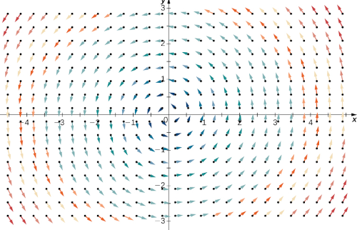
Answer: On the contrary! If we ob-serve a rotating asteroid, it will not only be information for us, but also a phenomenon that brings some energy and real consequences to it. This means that the operator:

\[ \vec{\nabla} = \vec{i}\frac{\partial}{\partial x} + \vec{j}\frac{\partial}{\partial y} + \vec{k}\frac{\partial}{\partial z} \]

has multiple uses. We call this operator nabla.

1. In addition to the divergence div(r) = \(\vec{\nabla} \cdot \vec{r}\) where nabla is the inner product of vectors, the same operator also defines the gradient:

\[ \text{grad}\ (f) = \vec{\nabla}f = \vec{i}\frac{\partial f}{\partial x} + \vec{j}\frac{\partial f}{\partial y} + \vec{k}\frac{\partial f}{\partial z}. \]

It also appears in the outer product of vectors as a rotor, or:

\[ \text{curl }\vec{v} = \vec{\nabla}\times \vec{v} = \begin{vmatrix} \vec{i} & \vec{j} & \vec{k} \\ \partial_x & \partial_y & \partial_z \\ v_x & v_y & v_z \end{vmatrix} = \] \[ = \vec{i}\left(\frac{\partial v_z}{\partial y} - \frac{\partial v_y}{\partial z}\right) + \vec{j}\left(\frac{\partial v_x}{\partial z} - \frac{\partial v_z}{\partial x}\right) + \vec{k}\left(\frac{\partial v_y}{\partial x} - \frac{\partial v_x}{\partial y}\right) \] \[ = [\vec{\partial}, \vec{v}]_x\vec{i} + [\vec{\partial}, \vec{v}]_y\vec{j} + [\vec{\partial}, \vec{v}]_z\vec{k}. \]

You can find details about vectors in my book Information Coupling.

2. Let's say that an asteroid or rock rotates around a vector \(\vec{\omega} = \omega\vec{k}\) that has a direction of the z-axis and an angular velocity ω, the intensity of that vector, then its points orbit in a plane parallel to the Oxy plane. A single point, which is \(\vec{r} = (x, y, z)\), thus moves with a velocity \(\vec{v} = \vec{\omega}\times \vec{r}\) always perpendicular to its radius vector \(\vec{r}\). Given that \(\vec{i}\times \vec{j} = \vec{k}\), \(\vec{j}\times \vec{k} = \vec{i}\), \(\vec{k}\times \vec{i} = \vec{j}\), and otherwise \(\vec{a}\times \vec{b} = -\vec{b}\times \vec{a}\) and \(\vec{a}\times\vec{a} = 0\), it will be:

\[ \vec{v} = \vec{\omega} \times \vec{r} = (\omega \vec{k}) \times (x\vec{i} + y\vec{j} + z\vec{k}) = -\omega y \vec{i} + \omega x \vec{j}. \]

So, we get a field like in the last picture on the left, and even before that we fo-und that the divergence of such a field is zero. However, the rotation exists:

\[ \text{curl }(\vec{v}) = \begin{vmatrix} \vec{i} & \vec{j} & \vec{k} \\ \partial_x & \partial_y & \partial_z \\ -\omega y & \omega x & 0 \end{vmatrix} = 2\omega\ \vec{k} = 2\ \vec{\omega}. \]

The rotor of points of a body rotating around a vector \(\vec{\omega}\), of arbitrary direction, is equal to twice that vector. The field of the previous answer in which the ar-rows dip into the starting point where the divergence of -2 was found would have a rotor of 0, because it does not rotate.

3. If a planet is in orbit, it does not fall towards the center of the gravitational field and vice versa, if a body does not fall into the center of gravity, it orbits. This is written in symbols where ∇ is a vector, f is a scalar and v is a vector:

∇ × (∇f) = 0,     ∇ ⋅ (∇ × v) = 0.

It is assumed that the nabla operator is the vector operator of the orthogonal vectors i, j and k are "ort-vectors", the unit vectors of abscissa, ordinate and applicate, so we often do not write the arrow above. Namely, the first follows from:

\[ \text{curl }(\text{grad }U) = \nabla \times (\nabla f) = \] \[ = \nabla \times \left(\frac{\partial f}{\partial x}\mathbf{i} + \frac{\partial f}{\partial y}\mathbf{j} + \frac{\partial f}{\partial z}\mathbf{k} \right) \] \[ = \left(\frac{\partial}{\partial y} \frac{\partial f}{\partial z} - \frac{\partial}{\partial z}\frac{\partial f}{\partial y}\right)\mathbf{i} + \left(\frac{\partial}{\partial z} \frac{\partial f}{\partial x} - \frac{\partial}{\partial x}\frac{\partial f}{\partial z}\right)\mathbf{j} + \left(\frac{\partial}{\partial x} \frac{\partial f}{\partial y} - \frac{\partial}{\partial y}\frac{\partial f}{\partial x}\right)\mathbf{k}. \]

However, equalities (Clairaut's Theorem) such as:

\[ \frac{\partial}{\partial y} \frac{\partial f}{\partial z} = \frac{\partial}{\partial z}\frac{\partial f}{\partial y}, \]

so the coefficients in front of the orthogonal vectors are zero and ∇ × (∇f) = 0. The second follows from:

\[ \text{div }(\text{curl }\mathbf{v}) = \nabla \cdot (\nabla \times \mathbf{v}) = \] \[ = \nabla \cdot \left( \left(\frac{\partial v_z}{\partial y} - \frac{\partial v_y}{\partial z}\right) \mathbf{i} + \left(\frac{\partial v_x}{\partial z} - \frac{\partial v_z}{\partial x}\right) \mathbf{j} + \left(\frac{\partial v_y}{\partial x} - \frac{\partial v_x}{\partial y}\right) \mathbf{k} \right) \] \[ = \frac{\partial}{\partial x}\left(\frac{\partial v_z}{\partial y} - \frac{\partial v_y}{\partial z}\right) + \frac{\partial}{\partial y} \left(\frac{\partial v_x}{\partial z} - \frac{\partial v_z}{\partial x}\right) + \frac{\partial}{\partial z} \left(\frac{\partial v_y}{\partial x} - \frac{\partial v_x}{\partial y}\right), \]

so, due to the equality of the expressions being subtracted in the parentheses, ∇ ⋅ (∇ × v) = 0.

4. Maxwell's equations (Information Coupling) describe the flow of electric curr-ent as an axis (vector) of rotation of a negative changing magnetic field or, co-nversely, magnetic current as an axis of rotation of a changing electric field:

curl(E) = -∂_tB,     curl(B) = ε₀μ₀∂_tE.

These are usually listed as the third and fourth, with the first two speaking of the absence of divergence in the two fields:

div(E) = 0,     div(B) = 0.

The solutions to Maxwell's equations are of the form:

\[ \mathbf{E} = \mathbf{E}_0\ e^{i(\mathbf{k}\cdot\mathbf{r} - \omega t)}, \quad \mathbf{B} = \mathbf{B}_0\ e^{i(\mathbf{k}\cdot\mathbf{r} - \omega t)}, \]

from which, by convention, the real part is taken for the physical solution. He-re E₀ and B₀ are constant vectors (of the electric and magnetic fields). Now k is not a "ort" vector, but a wave-vector, ω = 2πf is the angular frequency, whe-re the frequency f is the number of cycles per second. So k ⋅ r = ωt + 2nπ + φ, with some integer n and phase angle φ, the difference between the electric and magnetic fields.

5. Rotations are among the fundamental phenomena in science in general and certainly in this information theory. Oscillations are types of rotations, isome-tric transformations are too, and constancy is their basic characteristic, which is also an important property of "reality" (the definitions used here). Therefo-re, a rotating field is real, not just existing.

***

The text was completed on June 2, 2025.

July III 2025 (Original ≽)