July II 2025 (Original ≽)

In mathematics, an operator is a mapping from elements of one space to ele-ments of another space, usually of the same space. Here we mean linear ope-rators like this, A : X → X, from the vector space X to that same vector space. This imply a linear operator, A(αx + βy) = αA(x) + βA(y), where x and y are arbitrary vectors (from X), and α and β are any scalars (from Φ), usually real or complex numbers. Then we write Ax instead of A(x) for short.

Matrix II » srb

Question: Explain to me the matrix and its characteristic values, but slowly?

Answer: A manufacturer sells two types of ice cream at two locations. In the first location, the first type of ice cream brings in about 15 percent of the profit, while the second only 5 percent. However, in the second location, the first type of ice cream brings in 5 percent of the profit, and the second about 12 percent. He spends 100 cash points for the first type and about 110 for the second.

1. Let's put this description into the form of a system of linear equations:

\[ \begin{cases} a_{11}x_1 + a_{12}x_2 = y_1 \\ a_{21}x_1 + a_{22}x_2 = y_2 \end{cases} \]

At the first location, the profit coefficients are a₁₁ = 1.15 and a₁₂ = 1.05, and at the second location, a₂₁ = 1.05 and a₂₂ = 1.12, respectively. The investments for the first and second types of ice cream are x₁ = 100 and x₂ = 110 monetary units, so y₁ = 230.5 is the value of sales from the first location, and y₂ = 228.2 from the second.

2. Multiply the first equation by a₂₂, and the second by a₁₂, and subtract th-em. Again, multiply the first by a₂₁ and the second by a₁₁, and subtract them. We get:

\[ \begin{cases} (a_{11}a_{22} - a_{21}a_{12})x_1 = a_{22}y_1 - a_{12}y_2 \\ (a_{11}a_{22} - a_{21}a_{12})x_2 = a_{21}y_1 - a_{11}y_2 \end{cases} \]

On the left-hand sides we have the same factor, the determinant of the system. When we divide this system of equations by it, we can write it neatly:

\[ \begin{cases} b_{11}y_1 + b_{12}y_2 = x_1 \\ b_{21}y_1 + b_{22}y_2 = x_2 \end{cases} \]

Here, about b₁₁ = 6.04 and b₁₂ = -5.66, then b₂₁ = -5.66 and b₂₂ = 6.20. With these coefficients, we could calculate what the investment would be (x₁, x₂) if the gains (y₁, y₂) from selling ice cream were given.

3. We write the previous (1) system of linear equations in matrix form Ax = y, in more detail:

\[ \begin{pmatrix} a_{11} & a_{12} \\ a_{21} & a_{22} \end{pmatrix} \begin{pmatrix} x_1 \\ x_2 \end{pmatrix} = \begin{pmatrix} y_1 \\ y_2 \end{pmatrix}. \]

This defines the multiplication of the matrix A = (a_ij) by the vector x = (x_j) with indices i = 1, 2, ..., m and j = 1, 2, ..., n, and here m = n = 2. The inverse matrix is:

\[ A^{-1} = \frac{1}{\det A}\begin{pmatrix} a_{22} & -a_{12} \\ -a_{21} & a_{11} \end{pmatrix} = \begin{pmatrix} a'_{11} & a'_{12} \\ a'_{21} & a'_{22} \end{pmatrix}, \] \[ \det A = \begin{vmatrix} a_{11} & a_{12} \\ a_{21} & a_{22} \end{vmatrix} = a_{11}a_{22} - a_{21}a_{12} = 0.1855 \]

in the notation (2) where the coefficients of the matrix A^-1 = (a'_ij). Also, an inverse matrix exists iff its determinant is non-zero, only if det A ≠ 0.

Linear operators in general, and in particular matrices like this A, as well as arrays like these x and y, are special vector spaces. They can sometimes be assigned norms and metrics. Therefore, we are particularly interested in their interpretations and applications, and among the most important are process-like operators. Thus, this A is a process that translates the investment state x into the profit state y. Conversely, A^-1 would be some process by which we would find the value of the investment from the profit if its determinant were different from zero. The latter if and only if det A ≠ 0.

4. The eigenstate v of a given process A is the one in which the process does not change direction. This means Av = λv with some scalar λ, i.e. (A - λI)v = 0, where I is the identity matrix. In other words, det(A - λI) = 0, i.e.:

\[ \begin{vmatrix} a_{11} - \lambda & a_{12} \\ a_{21} & a_{22} - \lambda \end{vmatrix} = 0, \]

(a₁₁ - λ)(a₂₂ - λ) - a₂₁a₁₂ = 0,

λ² - (a₁₁ + a₂₂)λ + (a₁₁a₂₂ - a₂₁a₁₂) = 0,

λ² - tr(A)λ + (det A) = 0.

By tr(A) we denote the trace of the operator A. In the case of a matrix, this is the sum of its diagonal elements. Here we obtain two solutions:

λ₁ = 2.18511   and   λ₂ = 0.08489

Both are real numbers, because the given matrix is ​​symmetric, i.e. it is equal to its transpose, A^⊤ = A, with the columns replaced by rows. When we insert these eigenvalues ​​λ₁, then λ₂ into the characteristic equation Av = λv with v = (ξ, η), we find the corresponding eigenvectors:

\[ \begin{cases} 1.15 \xi + 1.05 \eta = \lambda \xi \\ 1.05 \xi + 1.12 \eta = \lambda \eta \end{cases} \]

Hence, approximately, when we normalize the eigenvectors with a 2-norm, when the sum of the squares of their coefficients is one:

\[ v_1 = \begin{pmatrix} 0.71214 \\ 0.70204 \end{pmatrix}, \quad v_2 = \begin{pmatrix} -0.70204 \\ 0.71214 \end{pmatrix}, \]

where the first eigenvector goes with the first eigenvalue, and the second with the second. Verify that Av_k = λv_k for both indices k = 1, 2.

5. Unlike “data,” what we call “information” is a quantity of options, a measure of uncertainty. However, due to the assumption of the ubiquity of information and the principle of minimalism, we also speak of data as (almost) zero infor-mation and its attractiveness. Therefore, facts, like natural laws, act as ancho-rs that dig into reality to bind other phenomena to themselves.

In this sense, the data we obtain with mathematical certainty are not some gr-eat information but are more significant to us as “gathering places.” Moreover, they themselves are often “carriers of possibilities.” There are various exampl-es of this. If v is the eigenvector of the eigenvalue λ of the operator A, then so is u = βv for every scalar β. Namely, from Av = λv, by multiplying by β ∈ Φ we get Aβv = λβv, or Au = λu, so u = βv is also the eigenvector of the eigenvalue λ of the operator A.

Scope » srb

Question: You mentioned “2-norm vectors” (Matrix II, 4). What is that?

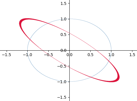
Answer: The image on the right is made by the program implicitly dr-awing two graphs. The first graph of the unit circle f₁ is blue. The se-cond graph is the red elliptic image of the given circle, f₂ = Af₁, with the matrix A of the previous example:

\[ A = \begin{pmatrix} 1.15 & 1.05 \\ 1.05 & 1.12 \end{pmatrix}. \]

The norm of a matrix is ​​the largest norm of the unit vector mapped by this A, the semi-major axis of the ellipse. This 2-norm of a vector and the farthest image of the unit circle as a 2-norm of a matrix uses the Pythagorean theorem and is sometimes impractical.

1. In probabilities, in the case of stochastic matrices (positive coefficients, unit column sums), in Markov chains, or in the aforementioned example when the sum (x₁, x₂) represents the total investment and the sum (y₁, y₂) represents the total profit, the 1-norm of the vector is more convenient. It is the simple sum of the absolute values ​​of the vector components, i.e., the largest of those in the columns of the given matrix.

Namely, from:

\[ \begin{pmatrix} a_{11} & a_{12} \\ a_{21} & a_{22} \end{pmatrix} \begin{pmatrix} x_1 \\ x_2 \end{pmatrix} = \begin{pmatrix} a_{11}x_1 + a_{12}x_2 \\ a_{21}x_1 + a_{22}x_2 \end{pmatrix}, \]

when |x₁| + |x₂| = 1, which is the "unit circle" of 1-norm, let us first consider only the positive vector components of the resulting vector and all its possible sums:

f(x₁) = [(a₁₁ + a₂₁) - (a₁₂ + a₂₂)]x₁ + (a₁₂ + a₂₂).

We are looking for the maximum of the function f(x₁) provided that x₁ ∈ (0, 1) and x₂ = 1 - x₁. This is the equation of the line that intersects the ordinate at the point a₁₂ + a₂₂ and whose tangent of the slope to the abscissa is the coefficient in front of x. When the tangent is positive, it is increasing and has the largest value f(1) = a₁₁ + a₂₁. This is the sum of the coefficients of the first column of the matrix. When the tangent is negative, it is decreasing and has the largest value f(0) = a₁₂ + a₂₂. This is the sum of the coefficients from the second column of the matrix.

This is the case of points from the first quadrant and condition |x₁| + |x₂| = 1. We find similarly for points II, then III and IV quadrants. The largest sum is always equal to the greater of the sum of the columns of the matrix. Therefore, the 1-norm of the matrix is ​​the largest value of the absolute sums of the coef-ficients of the columns of the matrix.

2. The dual of p-norms is q-norms, where p and q are positive ℝ numbers and the equality 1/p + 1/q = 1 holds. For the vector x₁ = (ξ₁, ξ₂, ..., ξ_n) then:

\[ \|x\|_p = \left(|\xi_1|^p + |\xi_2|^p + ... + |\xi_n|^p\right)^{1/p}. \]

We also denote this norm by L_p. In general, in my information theory, the rule is that an object that is in p-norm is perceived by a subject that is then in q-norm. Such a subject is then unique. The only such dual pairs are the numbers p = q = 2, and we have this in quantum mechanics. But then the coefficients of vectors and matrices are complex numbers, and the duals are adjoint (trans-posed and conjugated) vectors and matrices.

In tensor calculus, we often work with real numbers when the dual pairs are covariant and contravariant vectors (Variance), matrices, and tensors in gene-ral. Their products are invariants, they do not change with changing the coor-dinate system and therefore behave as "perception information". Thus, the corresponding perception of an object of L₁ norm belongs to L_∞ norm and vice versa, we perceive objects of L_∞ norm in the manner of L₁ norm. As we know, then for the above vector sequence:

\[ \|x_1\|_1 = |\xi_1| + |\xi_2| + ... + |\xi_n|, \] \[ \|x_1\|_\infty = \max\{|\xi_1|, |\xi_2|, ..., |\xi_n|\}. \]

This second norm is the limiting value when q → ∞.

3. That the L_∞ norm is indeed the absolute largest term, say ξ_k of the sequence x₁, can be seen when we extract it from before the parentheses:

\[ \|x_1\|_\infty = |\xi_k| \lim_{q \to \infty} \left(\frac{|\xi_1|}{|\xi_k|} + ... + \frac{|\xi_k|}{|\xi_k|} + ... + \frac{|\xi_n|}{|\xi_k|}\right)^{1/q} = |\xi_k|, \]

because sums of infinite powers, which are less than one, tend to zero.

In the case of a matrix, the L_∞ norm means calculating the sums of the abso-lute values ​​of its rows and taking the largest of them. This means that in ex-ample (1) above, we are looking for the (largest) value:

∥A∥_∞ = max{|a₁₁x₁ + a₁₂x₂| + |a₂₁x₁ + a₂₂x₂|},

taking the absolute greater of the numbers x₁ and x₂, which is then one, beca-use we are working with "unit circles," and the other is then zero. Thus it hap-pens that ∥A∥_∞ is greater among the absolute sums of the terms of the rows of the given matrix.

4. Let's look at what this means using the example of ice cream sales:

\[ Ax = \begin{pmatrix} 1.15 & 1.05 \\ 1.05 & 1.12 \end{pmatrix} \begin{pmatrix} 100 \\ 110 \end{pmatrix} = \begin{pmatrix} 230.5 \\ 228.2 \end{pmatrix} = y \]

The process A as an object has the value ∥A∥_∞ = 2.20. This is the sum of the elements of the first column of the matrix, which is greater than 2.17 of the sum of the second column. It so happens that in that very column there is also a larger element (1.15) that contributes to the largest sum of the total profit (230.5), which is not necessarily but is more likely. Therefore, the subject, ob-serving this process (matrix) as an object, measures the larger value of the sum of the rows and finds ∥A∥_∞ = 2.20 of the first row, which turned out to be indeed greater than the sum of the second row (2.17), which is more often the case, although it is not necessarily so.

The subject deals with the evaluations of objects and never with the values ​​of objects "in themselves," because such do not actually exist. Evaluations are al-ways different for different subjects, in different circumstances, and at differe-nt times. This is the meaning of Riesz's theorem, from which I get the proof of the uniqueness of information of perception.

Strategies » srb

Question: Does what you're telling me remind you of the minimax strategy?

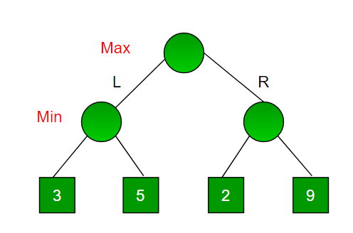
Answer: It makes sense to compare the L₁ and L_∞ norm matrices, espe-cially with so-called open games. Then two players alternately make moves as in a chess game, go, nim (taking objects from given piles), or tic-tac-toe. In the article on strate-gies, the minimax theorem is desc-ribed, which can be a good example for comparison. See also the link to the image on the left.

1. Let's imagine that Alice and Bob are playing a matrix game:

\[ M = \begin{pmatrix} 1 & 2 & 3 \\ 2 & 1 & 1 \\ 2 & 2 & 1 \end{pmatrix} \]

so that first Alice chooses a row so that Bob can choose a column and get the number of points in the intersection. Then Bob chooses a column so that Alice can choose a row and get the number of points in the intersection. Between moves, changes in the matrix numbers are possible, for example, random ones.

In the given arrangement, Alice will choose the second or third row first so that Bob cannot win 3 points but at most 2 if he chooses the column with a two. If Bob is first, he will not choose the third column so that Alice can ch-oose the row with at most 2 points. This is a minimax strategy that will give the consistent player the best chance of winning.

2. The conjugate values ​​of this matrix are different. The norm L₁ = 5, because all three columns have the same (absolute) sum of elements, and this is the maximum. And the norm L_∞ = 6, which is the sum of the elements of the first row, while the sum of the second is 4 and the third is 5. First of all, we note that ∥M∥₁ < ∥M∥_∞. In the norm of a vector, it is always ∥x∥_m ≤ ∥x∥_n whenever is 0 < m ≤ n ≤ ∞ (Lp Spaces).

Second, comparing the maximum row sum (L_∞ = 6) with the minimum (4), Alice has more choices than Bob, who has equal sums in each column (5). Roughly speaking, Alice can maneuver more in this move and make bigger mistakes through careless play. However, the value of the matrix is ​​too rough an estimate to be able to talk about the details and see a win in principle. That is the charm of the game, that the outcome is unpredictable.

3. We should understand this game as a distraction for the opponent. Players make moves so that their opponents do not have the best answers, because this makes sense with searching for a column (or row) with an absolute sum smaller than the norm ∥M∥₁ (i.e. ∥M∥_∞), the intensity matrix of the game. This can be verified in simulations (see Games).

For example, the computer generates a game matrix, such as M, and "Alice" chooses a row with a value less than M_∞, or any row if there is none, from which "Bob" will choose the (largest) element. Then, optionally, the computer somehow generates a game matrix so that "Bob" chooses a column with a value less than M₁, or any row if all values ​​are the same, from which "Alice" will choose the largest element. It is easy to do such simulations with vari-ations in the consistency of the players, and they will confirm the (statistical) accuracy of the above assumption.

4. Combinatorial games are typically contests between two opponents, with open moves and no elements of chance. For example, in addition to the above, there is the game dots and boxes in which multiple competitors can participa-te. Some card games, such as poker and bridge, do not fit the above definition and are classified as closed games. Even further from these are military, poli-tical, and many economic contests. Among these are "combinatorial" games with too many options or when there is too little time to make a move. I treat them in particular using "information perception".

Simulations III » srb

Question: Can you explain to me in detail how you test these games?

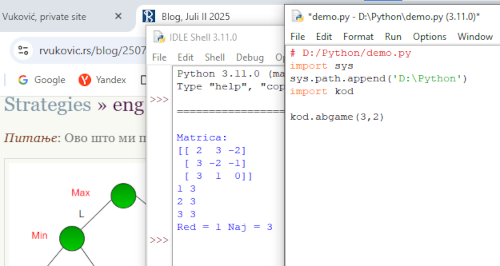
Answer: For example, I code simulations in the Python 3.11.0 progra-mming language in the image on the right. I work on them in their editor (Shell 3.11.0), in a special folder on my PC laptop. I write down the program (D:/Python/-demo.py) and that is my working demo for various calls of other pr-ograms or Python modules. You want details, so I describe the circumstances for those controversial Games.

In this case, the demo program contains only the following lines:

# D:/Python/demo.py
import sys
sys.path.append('D:\Python')
import kod

kod.abgame(3,2)

The first line is an internal comment (starting with # and not an executable command), followed by “import sys.” This is the activation of the module (sys) for various controls of parts of the Python environment. It is used here in particular to tell the program another, temporary, place to look for programs, with the following command: “sys.path.append('D:\Python')”. In the same folder there is also the program file “kod.py”, my module with many smaller modules. It is activated with “import kod.” Below, one of those submodules, “kod.abgame(3,2)” is called. I will explain it, and the detailed code is here.

This program, "kod.abgame(n, ind)" with parameters, is easy to modify. In this version, the first row is a square matrix n × n, the second is an indicator, one of the integers 0, 1, 2, 3. Here it will generate a 3 × 3 matrix with output to the screen, for example:

Matrica:
[[-1  2 -1]
 [-3  0  2]
 [-2  1  3]]
1 2
2 2
3 3
Red = 1 Naj = 2

The numbers in the matrix are random integers, from -n to n, and are differe-nt with each call to the program "abgame()". Below the matrix is ​​a printout of the rows and their maximum elements. At the bottom (Red = 1) is one of the possibly more optimal rows for the first player. The row has the smallest max-imum element, and from that the second player chooses the largest number (Naj = 2).

When we repeat the program many times (100,000) and add up the second player's points, they will cluster around 0.58 per cycle, for example like this:

# D:/Python/demo.py
import sys
sys.path.append('D:\Python')
import kod

zbir = 0
opet = 100000
for i in range(opet):
    naj  = kod.abgame(3,3)
    zbir = zbir + naj
print('Zbir =', zbir)

with the output “Zbir = 58479”. The average payoff of each of these moves was “zbir/opet = 0.58”. This is less than 1, and he could have an average of n = 3 points per cycle if he were without the first player's constraint. However, if the second player were to randomly pick a number from the square, his average would be 0. This is a confirmation of the von Neumann minimax theorem of game theory, using a simulation, in this case a game. By choosing moves so that the opponent does not have the best moves, we disable him to win.

The minimax theorem applies to games similar to this one, but only with a "saddle point." These are situations where the first player always has a row of the matrix (the first phase of the game's moves) without the largest number (the best answer) for the second player. This simulation proves that this pre-requisite is not necessary. It is enough that it appears occasionally; in a larger number of moves, the side that is less consistent in this choice and restriction will lose. This is an important step in confirming a different evaluation of str-ategies (Win Lose), which I use for other games.

Before continuing the current topic, about operators, I will also look at the observation of strategies using the information of perception. It is the scalar product of two sometimes very long sequences, or unusual functions, repre-senting the actions (information) of the subject and the object. So, functional. The larger this scalar, the greater the vitality of their coupling. We imagine it as the complexity of the possibility of choosing various game matrices for mi-nimax strategies. Disrupting the opponent is resistance to the negative, and choosing smaller rows is assistance to the good influence. As in a larger body composed of particles, a portion of the minimax properties is transmitted, and we have a simplified story about reciprocity as the preferred strategy.

Rectangular » srb

Question: Are the eigenvectors of the example (Matrix II, 4) with ice cream sales perpendicular and why are they?

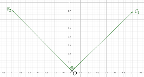
Answer: Yes, the eigenvectors v₁ and v₂ are orthogonal, because th-eir matrix A is symmetric. Incide-ntally, these two are also unitary, according to the L₂ norm:

∥v₁∥₂ = ∥v₂∥₂ = 1,

v₁ ⋅ v₂ = 0,     v₁ ⊥ v₂,

so they are orthonormal. It is assumed that all the members of the symmetric matrix are real numbers (a_ij ∈ ℝ) and equal to the transpose (a_ij = a_ji). We also write Â^* = Â and Â^⊤ = Â. A more general case of this is the Hermitian matrix. After conjugation and transposition, it is equal to itself, (Â^*)^⊤ = Â, so we say that it is self-adjoint and write Â^† = Â. A symmetric matrix is ​​a special case of a Hermitian matrix, so the assertion can be proven for the more general case.

1. We use Dirac notation (Bra-Ket), where ⟨v| means the adjoint, i.e. conjugate and transpose, of the vector |v⟩. Two characteristic equations of a Hermitian matrix are given: Â|u⟩ = α|u⟩ and Â|v⟩ = β|v⟩. Otherwise, α, β ∈ Φ are some scalars, usually real ℝ or complex numbers ℂ. However, these are the eigenva-lues ​​of the given matrix, precisely the scalars that go with the eigenvectors |u⟩ and |v⟩. Then α, β ∈ ℝ and, furthermore, if α ≠ β then ⟨v|u⟩ = 0.

2. Theorem. If Â|u⟩ = α|u⟩ and Â^† = Â, then α ∈ ℝ.

Proof: Multiplying the equality Â|u⟩ = α|u⟩ by the adjoint vector, we get:

⟨u|(Â|u⟩) = ⟨u|(α|u⟩) = α⟨u|u⟩ ∈ Φ.

By adjointing, then multiplying by the vector, the given equality gives:

(⟨u|Â)|u⟩ = (⟨u|α^*)|u⟩ = α^*⟨u|u⟩ ∈ Φ.

By comparison we find:

α⟨u|u⟩ = α^*⟨u|u⟩,

(α - α^*)⟨u|u⟩ = 0,

α - α^* = 0,

or α = α^*, and a number equal to its conjugate is real, i.e. α ∈ ℝ. ∎

3. In the case of a symmetric matrix, whose coefficients are real numbers, this proof is even shorter. From  = Â^⊤ = Â^* it follows that ⟨Âu|Âu⟩ = α²∥u∥², so since the left-hand side and the norm are real numbers, α² will be real, which means that α is a real number. Therefore, α ∈ ℝ.

4. That the eigenvectors of a real symmetric matrix are orthogonal, if they go along different eigenvalues, because ⟨Âu|v⟩ = ⟨u|Â^⊤v⟩, follows from:

β⟨v|u⟩ = ⟨βv|u⟩ = ⟨Âβ|u⟩ = ⟨v|Â^⊤u⟩ = ⟨v|Âu⟩ = ⟨v|αu⟩ = α⟨v|u⟩,

(β - α)⟨v|u⟩ = 0,

β - α ≠ 0   ⇒   ⟨v|u⟩ = 0,   v ⊥ u.

Therefore, the eigenvectors of a real symmetric matrix, with different eigen-values, are orthogonal.

5. Theorem. The eigenvectors of a Hermitian matrix, which have different eigenvalues, are orthogonal.

Proof: From Â|u⟩ = α|u⟩ follows ⟨u|Â = ⟨u|α, for α ∈ ℝ. Also Â^† = Â, and:

(⟨u|Â^†)|v⟩ = ⟨u|(Â|v⟩),

(⟨u|α)|v⟩ = ⟨u|(β|v⟩),

α⟨u|v⟩ = β⟨u|v⟩,

(α - β)⟨u|v⟩ = 0,

α - β ≠ 0   ⇒   ⟨u|v⟩ = 0,   |u⟩ ⊥ |v⟩.

This completes the proof. ∎

What is the benefit of this, of the orthogonality of the eigenvectors of the pr-ocess, is the unstated second part of the question above. There are so many applications of it that the answer to that part of the question is a separate topic. Let us recall, for example, measurement starting from quantum mec-hanics.

Fictitious » srb

Question: What processes are fictitious, are there linear operators that descri-be such processes?

Answer: I have given examples of such (Null Space II), non-zero ma-trices that map vectors of a certain set, their non-empty "null space", to zeros.

We know that every system of equ-ations

\[ \begin{cases} a_{11}x_1 + a_{12}x_2 = 0 \\ a_{21}x_1 + a_{22}x_2 = 0 \end{cases} \]

In general, Ax = 0, written in matrix form, has a trivial solution x₁ = x₂ = 0. However, if the determinant of A is zero, it also has non-trivial solutions. Then there are vectors, x ≠ 0, sequences that also have non-zero elements. The rank of that matrix is ​​less than the order.

These examples follow the new definition of reality (noticability, permanence, and truth), a feature of this theory. Fictional phenomena are phenomena that lack one or two of the properties of reality. When they are not "noticable," the impossibility of indirect communication is implied, when the vector space is wider than the one they span. If they do not have "permanence," then the pr-ocesses that are extinguished are part of the world of untruth, not a physical one with laws of conservation. This, briefly, is an introduction to what follows.

1. The determinant of a matrix (operator) measures the hypervolume of the space spanned by its column vectors. Thus, the surface of a 3-dimensional sp-ace is of zero "volume," i.e., a third-order matrix (of type 3×3) whose columns are not linearly independent vectors has a determinant of zero. Hence we have det(A - λI) = 0 for the characteristic equality Av = λv, when λ is an eigenvalue of the matrix A with its eigenvector v, because Av - λv = 0, hence (A - λI)v = 0, which means that v is from the zero space of the matrix A - λI.

On the other hand, from every matrix A whose determinant is not zero, acco-rding to what has been said, we can extract the diagonal matrix λI and from v, the eigenvector of that matrix, we have the null-space vector of matrix A - λI. Expressed in this way, this well-known statement of linear algebra has a new meaning: there are fictions everywhere.

2. A lie is attractive but not permanent. It easily becomes desirable, and if we become attached to it, we protect it with force; it becomes a useful expense. If we follow the truth, however, we do not have a problem of permanence but of the power of those who are addicted to the lie. As real information of laws, a lie is equally diluted and attractive by the principle of minimalism, except that it lives on borrowed strength.

Deep beneath this life story lie the ladder operators (Ladder II):

\[ \hat{a}^- = \begin{pmatrix} 0 & \sqrt{1} & 0 & ... \\ 0 & 0 & \sqrt{2} & ... \\ 0 & 0 & 0 & ... \\ ... \end{pmatrix}, \quad \hat{a}^+ = \begin{pmatrix} 0 & 0 & & ... \\ \sqrt{1} & 0 & 0 & ... \\ 0 & \sqrt{2} & 0 & ... \\ ... \end{pmatrix}. \]

These are the matrices of descent (annihilation) and ascension (creation), wh-ich are infinite due to the absence of energy constraints on the upper side. It is easy to see that their determinants are zero. They themselves are unfinished processes, but their sum and difference define the position and momentum operators:

\[ \hat{x} = \sqrt{\frac{\hbar}{2m\omega}}(\hat{a}^+ + \hat{a}^-), \quad \hat{p} = i\sqrt{\frac{\hbar m\omega}{2}}(\hat{a}^+ - \hat{a}^-) \]

whose interpretations are real phenomena of quantum mechanics.

3. In the case of finite matrices, it is useful to know the characteristic polyno-mial of the operator. This is the determinant det(A - λI) = 0, i.e.:

f(λ) = det(A - λI) = a₀ + a₁λ + a₂λ² + ... + a_n-1λ^n-1 + λⁿ

where n ∈ ℕ is the order of the operator and its matrix A. For matrices of rank less than order, when its columns (rows) are linearly dependent vectors, the constant sum of this polynomial is zero. Namely, f(0) = det(A) = 0, so a₀ = 0. At least one of the eigenvalues ​​is then λ = 0.

Here are more examples. According to Vieta's formulas, a₁ = λ₁ + ... + λ_n, which is the trace of the matrix, the sum of all its eigenvalues. They also confirm the previous one, since det(A) = λ₁⋅...⋅λ_n and establish that a₀ is the product of the eigenvalues. When the matrix A is real and n is odd, λⁿ for large |λ| is a dominant sum. Then f(λ) < 0 if λ < 0, but f(λ) > 0 for λ > 0, which means that the graph f(λ) intersects the abscissa and the matrix has at least one real eigenvalue, λ ∈ ℝ.

No matter what the matrix A is, if it has some real eigenvalue λ, then there exists a real column vector u ≠ 0 such that Au = λu. Namely, then Aw = λw and if some members of the column vector w are complex numbers, we separate them into real and imaginary parts, w = u + iv, of the real column vectors u and v. From A(u + iv) = λ(u + iv), equating the two sides of the real and imaginary parts, we find Au = λu and Av = λv.

4. Not all (linear) operators of the zero determinant are some fiction, nor are all fictions of that form. After all, fictions are just a phenomenon that is not re-al. I would not like to predict where this completely new theory might extend, but it seems inspiring enough for development, and a better answer to the question will have to wait.

Plagiarism » srb

Question: Where do you find those examples of matrices with such convenient eigenvectors?

Answer: The question is more rela-ted to other, more professional cor-respondences and not to this kind of blog. However, I could edit the answer for an easier opportunity, I hope.

1. The first way is to search the In-ternet, but I avoid that. There are many software programs that will instantly detect plagiarism, and re-aders could easily think that in addition to the examples, you are also stealing intellectual property and that they would be better off looking for originals. Colleagues see you as a fraud, and you are deprived of the experience of crea-tivity. It's not worth the speed it seems, and when it's justified, like the attac-hed image on the top left (drawing is not the topic here), I put a link to the origin.

2. Another way is to guess. You choose a problem and form a matrix that you then solve as I mentioned above (Matrix II), and see what comes out. This procedure was asked of me in the question (Projection II), because it is com-mon in linear algebra classes. It is not practical, because a good guess is un-likely, but there are special situations when it is desirable.

3. I use the third method even more often. It is rarer otherwise, and you will need a comment attachment. You choose any set of n ∈ ℕ column vectors, ea-ch with n members that are, to begin with, mutually orthogonal. At the same time, you choose any sequence of n numbers. The vectors are, say, v₁, ..., v_n, and the numbers λ₁, ..., λ_n. The auxiliary matrix P = P[v₁, ..., v_n] will be a squ-are of order n, because its columns are precisely the selected vectors, and the diagonal D = D(λ₁, ..., λ_n) on the diagonal it has the selected numbers in the given order and all other elements zero.

Then we normalize the vectors v_k, dividing each by its intensity to obtain an orthonormal set of vectors. Then the adjoint (conjugate and transpose) matrix P is exactly its inverse, P^† = P^-1, because by multiplying P by P^⊤, or in reverse order, we are scalarly multiplying a column either by its conjugate when the result is 1, or by some other orthogonal column to it when the result is 0. The product is the identity matrix, PP^⊤ = P^⊤P = I.

The triple product A = PDP^-1 will be a matrix with eigenvalues ​​chosen λ_k with linked eigenvectors v_k, respectively for k = 1, ..., n. Namely, Av_k = PDP^-1v_k, but the first multiplication P^-1v_k gives a column vector with 1 in the k-th row and all other zeros, which the second multiplication with D translates into a colu-mn vector with the number λ_k in the k-th row and all other zeros. This multip-lied by P will give λ_kv_k. It turns out Av_k = λ_kv_k, i.e. λ_k is an eigenvalue of A and the corresponding eigenvector is v_k.

4. Here is an example of the method (A = PDP^-1) with two orthogonal vectors:

\[ A = \begin{pmatrix} a & -b \\ b & a \end{pmatrix} \begin{pmatrix} \alpha & 0 \\ 0 & \beta \end{pmatrix} \cdot\frac{1}{a^2 + b^2} \begin{pmatrix} a & b \\ -b & a \end{pmatrix}, \] \[ A = \frac{1}{a^2 + b^2} \begin{pmatrix} \alpha a^2 + \beta b^2 & (\alpha - \beta)ab \\ (\alpha - \beta)ab & \beta a^2 + \alpha b^2 \end{pmatrix}, \]

in real space (a, b, α, β ∈ ℝ). When a² + b² = 1, the columns of the auxiliary matrix P[v₁, v₂] are the orthonormal basis of the 2-dim space. Anyway, it is:

\[ Av_1 = \begin{pmatrix} a & -b \\ b & a \end{pmatrix} \begin{pmatrix} \alpha & 0 \\ 0 & \beta \end{pmatrix} \cdot \frac{1}{a^2 + b^2} \begin{pmatrix} a & b \\ -b & a \end{pmatrix} \begin{pmatrix} a \\ b \end{pmatrix} = \] \[ = \begin{pmatrix} a & -b \\ b & a \end{pmatrix} \begin{pmatrix} \alpha & 0 \\ 0 & \beta \end{pmatrix} \cdot \frac{1}{a^2 + b^2} \begin{pmatrix} a^2 + b^2 \\ 0 \end{pmatrix} \] \[ = \begin{pmatrix} a & -b \\ b & a \end{pmatrix} \begin{pmatrix} \alpha & 0 \\ 0 & \beta \end{pmatrix} \begin{pmatrix} 1 \\ 0 \end{pmatrix} \] \[ = \begin{pmatrix} a & -b \\ b & a \end{pmatrix} \begin{pmatrix} \alpha \\ 0 \end{pmatrix} = \begin{pmatrix} \alpha a \\ \alpha b \end{pmatrix}, \] \[ \frac{1}{a^2 + b^2} \begin{pmatrix} \alpha a^2 + \beta b^2 & (\alpha - \beta)ab \\ (\alpha - \beta)ab & \beta a^2 + \alpha b^2 \end{pmatrix} \begin{pmatrix} a \\ b \end{pmatrix} = \alpha \begin{pmatrix} a \\ b \end{pmatrix}, \]

i.e. Av₁ = αv₁. Check similarly Av₂ = αv₂, or by directly multiplying the last term. For example, A = PDP^-1 is:

\[ \frac{1}{25}\begin{pmatrix} 41 & -12 \\ -12 & 34 \end{pmatrix} = \begin{pmatrix} 3 & -4 \\ 4 & 3 \end{pmatrix} \begin{pmatrix} 1 & 0 \\ 0 & 2 \end{pmatrix} \cdot \frac{1}{25}\begin{pmatrix} 3 & 4 \\ -4 & 3 \end{pmatrix} \]

and here is an example of a matrix A with convenient eigenvectors v₁ and v₂. Now we see how far the arbitrariness of these vectors can go for the same ma-trix A, and especially how much greater the choice of eigenvalues ​​α and β can be for always the same eigenvectors of that same matrix.

5. There is a proverb that even a sheet of paper has two sides. This is true for “freedom,” S = I⋅H, the product of “intelligence” and “hierarchy” of slightly broader concepts than usual (Completion), which reaches its maximum when its factors are equal, and so it is with “knowledge” and “creativity,” where the first would be algebraic skills like the ones mentioned, and the second their use in unexpected findings, scientific discoveries. It is a loss to neglect the second for the sake of the first, or vice versa.

By tireless study at the university, opportunities can be wasted, or the brain can be overtrained on the familiar things it otherwise loves most, completely losing its ability to penetrate the unknown. It suppresses feelings that are much greater than the joy of discovery. On the other hand, the pleasure of children's play can overwhelm us and deprive us of the desire to learn about the centuries-old discoveries of geniuses greater than us, laborious for us at the time, but without which we easily remain charlatans in the domain of science. I am trying to explain the formula S = H⋅I for this case.

Induction » srb

Question: I noticed that you rarely use mathematical induction. Do you consi-der it a bad method, impractical?

Answer: I use mathematical indu-ction (Transitions, 4), perhaps not enough as it is common, useful, and accurate in applications, so here are more examples.

1. Theorem. Let v₁, v₂, ..., v_n be the eigenvectors of the matrix A and their corresponding all distinct eigenvalues ​​λ₁, λ₂, ..., λ_n. Then the set v_k for k = 1, 2, ..., n constitutes linearly independent vectors.

Proof: It is clear that this statement is true for n = 1. Suppose that for the nu-mber m ≥ 2, α₁v₁ + α₂v₂ + ... + α_mv_m = 0 for some scalars α₁, α₂, ..., α_m. It will be:

α₁Av₁ + α₂Av₂ + ... + α_mAv_m = 0,

so it is:

α₁λ₁v₁ + α₂λ₂v₂ + ... + α_mλ_mv_m = 0.

Multiplying the first of these equalities by λ₁ and subtracting the second from it, we have:

(λ₁ - λ₂)α₂v₂ + ... + (λ₁ - λ_m)α_mv_m = 0.

By the induction hypothesis, if v₂, ..., v_m are linearly independent, then it is (λ₁ - λ_k)α_k = 0 for each k = 2, ..., m. Since λ₁ ≠ λ_k for all k = 2, ..., m, must be each α_k = 0. Thus, α₁ = 0 and v₁, v₂, ..., v_n are linearly independent. ∎

2. When a matrix is ​​symmetric, or is complex and therefore Hermitian, then its eigenvalues ​​are real, and the associated eigenvectors are mutually orthogo-nal (Rectangular). However, this theorem states that the eigenvectors of diffe-rent eigenvalues ​​are linearly independent. They need not be orthogonal if the matrix is ​​not Hermitian (if it is real, as soon as it is Hermitian, it is symmetr-ic). For example:

\[ \begin{pmatrix} 1 & 2 \\ 5 & 4 \end{pmatrix}\begin{pmatrix} 1 \\ -1 \end{pmatrix} = -\begin{pmatrix} 1 \\ -1 \end{pmatrix}, \quad \begin{pmatrix} 1 & 2 \\ 5 & 4 \end{pmatrix}\begin{pmatrix} 2 \\ 5 \end{pmatrix} = 6\begin{pmatrix} 2 \\ 5 \end{pmatrix}, \]

which is easy to check by multiplication. The given matrix is ​​not symmetric; its eigenvalues, ​​-1 and 6, are distinct real numbers, and the corresponding eigenvectors are not orthogonal but "only" linearly independent.

3. Hermitian operators define the "observables" of quantum mechanics as wave functions (Measurement II):

\[ |\alpha\rangle = \sum_k \alpha_k |v_k\rangle, \quad \alpha_k = \langle v_k | \alpha\rangle. \]

whose squares of the modulus, |α_k|², of the coefficients of the factors of indi-vidual basis vectors, |v_k⟩, are the probability of finding in the measurement exactly k-th observable of a given operator. This is the meaning of the ortho-gonality of these basis, eigenvectors of the operator (according to my inform-ation theory), i.e. the described Hermitianity. Their eigenvectors are mutually orthogonal, so that by measuring one of them, the projections onto all the oth-ers will be zero, so the entire superposition collapses into a single outcome.

In the case of non-Hermitianity, or asymmetry of the macro-state, as we see in the previous example (2), there is no collapse of everything into a single outco-me, so the superposition breaks down into multiple "observables".

4. In the example of the previous answer (Plagiarism, 4), for the same α = β, eigenvalues ​​of the matrix A, but a ≠ b we have the same general orthogonal eigenvectors v₁ = (a, b)^⊤ and v₂ = (-b, a)^⊤ which form the basis of some 2-dim space. This happens whenever the eigenvalues ​​of an operator in general are repeated. Imagine that we have a sequence of eigenvalues ​​λ₁, λ₂, ..., λ_j, each of which is repeated in the order μ₁, μ₂, ..., μ_j times, forming bases P₁, P₂, ..., P_j with as many vectors as the number of times the eigenvalue is repeated. The union of all these bases, P = P₁ ∪ P₂ ∪ ... ∪ P_j, is a set of linearly independent vectors. It is proved as in Theorem (1), from which it follows that there exists a diagonal matrix D such that A = PDP^-1.

Otherwise, the basic matrix diagonalization theorem states that a matrix A of type n×n can be written in the form A = PDP^-1 if and only if it has exactly n li-nearly independent eigenvectors. Then the eigenvectors are the columns of the auxiliary matrix P, and the elements of the diagonal matrix D have the corres-ponding eigenvalues ​​given by the order of the columns. A different arrangem-ent of the columns of P will give a different diagonalization order D = P^-1AP.

Multiplicity » srb

Question: What are algebraic and geometric multiplicity and how do they differ?

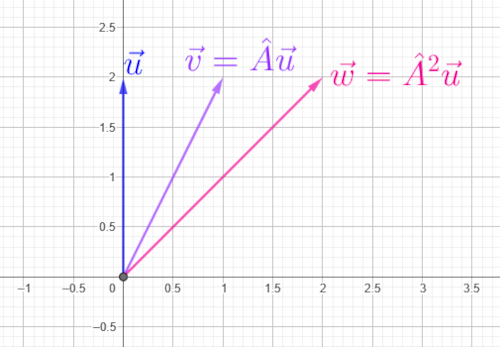
Answer: The algebraic multiplicity of a scalar λ ∈ Φ is its multiplicity as a root of the characteristic poly-nomial of an operator, or its matrix A. The geometric multiplicity of λ is the dimension of the λ-eigenspace.

1. Shear operators along one of the axes are often given in the literatu-re as simple examples for the diffe-rences between these two manifo-lds. Here is an example of such a shear along the first axis in the plane Au = v, in detail:

\[ \begin{pmatrix} 1 & 1 \\ 0 & 1 \end{pmatrix} \begin{pmatrix} x \\ y \end{pmatrix} = \begin{pmatrix} x + y \\ y \end{pmatrix}. \]

In the image on the left, you see the operator A moves the point u = (0, 2) to the point v = (1, 2), and by repeated action, this to the point w = (2, 2). I use various notations, otherwise common everywhere, so you can find them easier to use in applications.

This operator does not make changes along the second axis, it is 1-dim, so it has geometric multiplicity 1. However, the eigenvalue λ of the characteristic equation Av = λI, i.e. the number of its multiplicity in the (Fictitious, 1) pol-ynomial det(A - λv) = 0, is 2. Namely:

\[ \begin{vmatrix} 1 - \lambda & 1 \\ 0 & 1 - \lambda \end{vmatrix} = 0, \]

(1 - λ)² = 0,

λ₁ = λ₂ = 1.

A double root of a characteristic polynomial means that 2 is the algebraic multiplicity of the scalar λ.

The only non-zero eigenvector of this operator, its matrix A, is the unit abscissa vector. We find this from Av = λv, more precisely:

\[ \begin{pmatrix} 1 & 1 \\ 0 & 1 \end{pmatrix} \begin{pmatrix} x \\ y \end{pmatrix} = 1\cdot \begin{pmatrix} x \\ y \end{pmatrix}, \] \[ \begin{cases} x + y = x \\ y = y \end{cases} \]

x₁ = 1, y₁ = 0   и   x₂ = y₂ = 0.

These are the column vectors v₁ = (1, 0)^⊤ and v₂ = (0, 0)^⊤. The position on the abscissa moves 1 to the right with each action of A while the position on the ordinate remains stationary.

2. The column space of the shear matrix is ​​of dimension 2. This is also seen fr-om its determinant, det(A) = 1, which is nonzero, meaning that the "volume" of 1 spanned by its two columns is nonzero. In a matrix of row 2, its two colu-mns form linearly independent vectors if its determinant is nonzero. In gene-ral, the determinant is nonzero if the row of the matrix (the number of colum-ns) is equal to the rank of the matrix (the number of linearly independent co-lumns).

Therefore, in the equality A = PDP^-1, where P is the column matrix of eigenve-ctors of the matrix A, and D is the diagonal matrix of eigenvalues ​​of that matr-ix, if det(A) = 0, then det(PDP^-1) = 0. But the determinant of the product is eq-ual to the product of the determinants, so then:

det(PDP^-1) = det(P)⋅det(D)⋅det(P^-1) = det(PP^-1)⋅det(D) = det(D) = 0,

which means that some of the eigenvalues ​​(on the diagonal of the matrix D) are zero, i.e., that the matrix A does not have a diagonal matrix. In other wor-ds, we have contradicted the assumption that there is an equality A = PDP^-1. The matrix cannot be diagonalized if the algebraic multiplicity of the scalar λ is not equal to its geometric multiplicity! This conclusion is equivalent to the previous one (Induction, 4), although achieved in a different way.

3. The diagonal elements of a triangular matrix are its eigenvalues. Thus, the following matrix, A, has two unequal eigenvalues ​​λ₁ = 1 and λ₂ = 3 with corr-esponding eigenvectors v₁ and v₂:

Av₁ = λ₁v₁,     Av₂ = λ₂v₂,

\[ \begin{pmatrix} 1 & 2 \\ 0 & 3 \end{pmatrix} \begin{pmatrix} 1 \\ 0 \end{pmatrix} = \begin{pmatrix} 1 \\ 0 \end{pmatrix}, \quad \begin{pmatrix} 1 & 2 \\ 0 & 3 \end{pmatrix} \begin{pmatrix} 1 \\ 1 \end{pmatrix} = 3 \begin{pmatrix} 1 \\ 1 \end{pmatrix}, \]

which are linearly independent, because det(A) ≠ 0, but are not orthogonal. Although this matrix is ​​not symmetric (Induction, 2), it has a diagonal:

\[ \begin{pmatrix} 1 & 2 \\ 0 & 3 \end{pmatrix} \begin{pmatrix} 1 & 1 \\ 0 & 1 \end{pmatrix} = \begin{pmatrix} 1 & 1 \\ 0 & 1 \end{pmatrix} \begin{pmatrix} 1 & 0 \\ 0 & 3 \end{pmatrix}, \]

AP = PD,

A = PDP^-1,

where the auxiliary matrix P = P[v₁, v₂] has columns that are the eigenvectors of the matrix A and whose corresponding eigenvalues ​​are on the diagonal D. The algebraic multiplicity of the scalar λ is 2, and the geometric multiplicity of λ is also 2, since the corresponding eigenvectors span a space of dimension 2.

4. The eigenvalues ​​of observed observables are real because they are possible measurement outcomes of a given notice. The corresponding eigenvectors, or eigenstates, span the Hilbert space. This means that the observables generate orthonormal bases, i.e., they are elements of a linear combination of the eigen-vectors and the measurement states. We know this, and the question is: what about eigenvalues ​​that are not real?

Thus, the rotation matrix (θ = π/2) has no real eigenvalues:

\[ A(\pi/2) = \begin{pmatrix} 1 & -1 \\ 1 & 1 \end{pmatrix} \begin{pmatrix} \pm \frac{i}{\sqrt{2}} \\ \frac{1}{\sqrt{2}} \end{pmatrix} = (1 \pm i)\begin{pmatrix} \pm \frac{i}{\sqrt{2}} \\ \frac{1}{\sqrt{2}} \end{pmatrix}. \]

These are two equations, the first has "+" in three places "±", and the second has "-" in three places, where i² = -1. When these are the characteristic equati-ons Av₁ = λv₁ and Av₂ = λv₂, then A is a rotation, the eigenvalues ​​λ₁₂ = e^±iθ, the corresponding eigenvectors are v₁₂ = (±i, 1). Linear combination of eige-nvectors:

v = α₁v₁ + α₂v₂,     α₁, α₂ ∈ ℂ,

are states that can be measured, each with its own probability by the square of the modulus, such that |α₁|² + |α₂|² = 1.

Rotation III » srb

Question: You've stopped the story (Multiplicity, 4) at the most interesting po-int in the rotations. What's the problem?

Answer: Rotations are not so much a “problem” within my private rese-arch on information as they might be outside, and I tend to forget th-at. For example, the question that is the subject of the image link on the right (2022) I have considered before, for example, in tensor mod-els of the universe (Rotating Unive-rse, 2014), also viewing parts of the gravitational field as rotations (Six Dimensions, 2015), often performing rota-tions in my own way, using a commutator, which emphasizes their informati-onal nature. That's why I tested many other models of the universe (Metric of the Torus, 2016).

1. Rotation matrix:

\[ A(\theta) = \begin{pmatrix} \cos\theta & -\sin\theta \\ \sin\theta & \cos\theta \end{pmatrix} \]

has det(A) = 1, eigenvalues ​​λ₁₂ = e^±iθ = cos(θ) + i sin(θ) and associated eigen-vectors:

\[ v_1 = \begin{pmatrix} \frac{i}{\sqrt{2}} \\ \frac{1}{\sqrt{2}} \end{pmatrix}, \quad v_2 = \begin{pmatrix} -\frac{i}{\sqrt{2}} \\ \frac{1}{\sqrt{2}} \end{pmatrix}, \]

which form an orthonormal basis of the 2-dim space of their matrix. This is easily verified by direct matrix multiplication Av₁ = e^iθv₁ and Av₂ = e^-iθv₂. However, it (λ₁₂ ∉ ℝ) indicates that rotation is not a physics of reality.

2. How is it possible that there is nothing that we all witness every day? Nice, because rotation is not what we think it is. Besides, it is not that it does not exist; it is just said that rotation is not observable. For example, when I look at you while you look at yourself (Different) we are not looking at the same phen-omenon. This is due to the limited speed of light and distance. While I see yo-ur past, you are already in other presents. The distances between body parts also separate personal presents.

Given objective coincidence (a principle from my information theory), he was not really "exactly the same" as I see "him" in the past, and these are already two reasons for the questionability of what we are witnessing. The third type of ravel arises from the slowing down of the flow of time in general for a body in motion. A rotating position has a slower time the further it is from us (to the center) because its speed of circulation is higher. Decreasing speeds of ti-me relative to the center of rotation, they are also different from each other, excluding the relativity of motion.

From this, it follows that the imaginary rotating system is a "middle-earth" or a "lodge neither in heaven nor on earth." It is neither present nor part of the space we see, which is the repository of the past of the celestial bodies we observe.

3. The solutions of the characteristic equation Av = λv will be the eigenvalues ​​of the λ operator, i.e. the matrix A. This reduces to (A - λI)v = 0, i.e. to the nu-ll-space of the A - λI operator, which is not empty because v ≠ 0, which means that det(A - λI) = 0. Thus, finding the eigenvalue of the operator reduces to so-lving the so-called minimal polynomial of the operator. If we work with a real matrix A, we will have a polynomial of the variable λ with real coefficients that has at least one real root, if it is of odd degree.

In other words, a third-order matrix has at least one real eigenvalue and does not have the problem that we have with rotation. Again, this means that rota-tion is a 2-dim phenomenon and is not something that we would like to see as the universe spreading out in all directions due to centrifugal force. These are excerpts from some of the texts mentioned above that I dealt with about 10 ye-ars ago. They further lead to a completely new attempt, to such unusual consi-derations of connecting rotation with principled minimalism, that I hardly da-re to talk about it.

4. We know from social life that lies are attractive to us, and here I interpret them as diluted uncertainty, and, according to the broad tendency towards more probable states, or less informative and smaller physical actions, lies and fiction in general also approach reality. Not simply because the hill goes to me when I go to the hill (I am wary of claiming that the laws of fiction are the laws of physics), but because with reality, fiction lasts longer, and by simple selecti-on, there will be more of it. Still, the slowed-down flow of time created by rota-tion is attracted to the axis of rotation and does not let go easily.

With more mass, the axis has more reality and more appeal. It is one of my longest-running (hypo)theses, from then and about this problem. I emphasize that I have not dealt with it much, but it "holds water" and, incidentally, expla-ins a lot of things in physics. For example, angular momentum. Attracted by a force that exists only because it is spinning, the object continues to spin. I wo-uld say more, but maybe this is too much.

Teaching » srb

Question: I would like to see some interesting example of the application of rotations and eigenvalues, if possible, for teaching to my students?

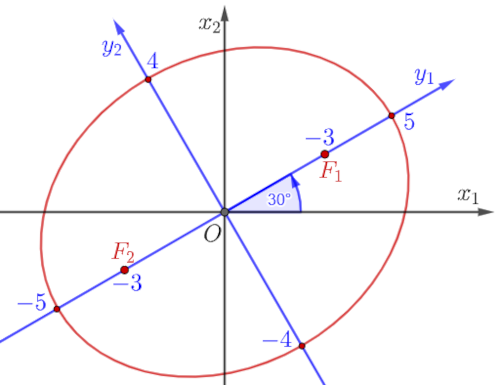
Answer: Show them the formulas (Plagiarism, 4). Give examples of their application to conics, as in the figure on the left. In general, then a = cos(θ) and b = sin(θ), and the eigenvalues ​​α and β are the two (i.e. major and minor) semiaxes of the ellipse.

1. The eigenvectors are then:

\[ v_1 = \begin{pmatrix} \cos\theta \\ \sin\theta \end{pmatrix}, \quad v_2 = \begin{pmatrix} -\sin\theta \\ \cos\theta \end{pmatrix}. \]

The auxiliary matrix is ​​the rotation:

\[ P = \begin{pmatrix} \cos\theta & -\sin\theta \\ \sin\theta & \cos\theta \end{pmatrix}, \]

and the target matrix of the operator is:

\[ A = \begin{pmatrix} (\alpha - \beta)\cos^2\theta + \beta & (\alpha - \beta)\cos\theta\sin\theta \\ (\alpha - \beta)\cos\theta\sin\theta & \beta + (\alpha - \beta)\sin^2\theta \end{pmatrix}. \]

It is a matrix that stretches the unit circle of the rectangular Cartesian coordi-nate system Ox₁x₂ into the ellipse of the system Oy₁y₂.

2. For example, as in the given figure, the major semi-axis of the ellipse α = 5, the minor β = 4, and the rotation angle θ = 30°. It is known that cos(30°) = √(3)/2 and sin(30°) = 1/2, so:

\[ A = \begin{pmatrix} \frac{19}{4} & \frac{\sqrt{3}}{4} \\ \frac{\sqrt{3}}{4} & \frac{17}{4} \end{pmatrix}. \]

Such A is an operator of stretching the abscissa (in the figure the x₁-axis) five times (α = 5), and the ordinate (x₂-axis) four times (β = 4) and rotating the system (Ox₁x₂ → Oy₁y₂) by θ = 30°. The eigenvectors are the directions of the stretching.

3. Check: We solve the polynomial operator det(A - λI) = 0, step by step:

\[ \begin{vmatrix} \frac{19}{4}-\lambda & \frac{\sqrt{3}}{4} \\ \frac{\sqrt{3}}{4} & \frac{17}{4} - \lambda \end{vmatrix} = 0, \] \[ \left(\frac{19}{4} - \lambda\right) \left(\frac{17}{4} - \lambda\right) - \frac{3}{16} = 0, \]

16λ² - 4(19 + 17)λ + 19⋅17 - 3 = 0,

16λ² - 144λ + 320 = 0,

λ² - 9λ + 20 = 0,

λ₁ = 5,     λ₂ = 4.

These are indeed the given eigenvalues. I recommend both this and the verification by direct matrix multiplication Av = λv for teaching.

Mixture » srb

Question: Can you reduce the problem of "dilution" of present information to, say, differential equations?

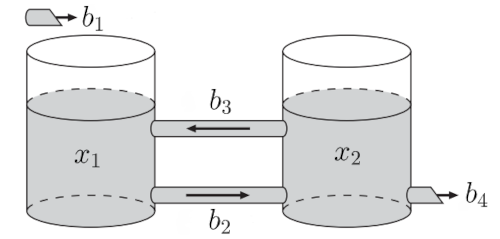
Answer: This is a question of deba-te about the definition of "reality", which, among other things, has du-ration, therefore also a past, and on top of that is the law of preservati-on. The present "melts" into the tr-ace of the past, which it somewhat complements, so that the total am-ount of uncertainty rest unchanged.

1. We talk about information (amount of uncertainty) as a salt solution in wat-er in order to use a typical system of linear differential equations and the mod-el shown in the figure on the right. For example, with b₁ a new uncertainty ar-rives in the present of the quantity x₁. This part b₂ goes to the past where it al-ready exists x₂ from which b₃ returns to it, and b₄ is irretrievably lost. Short:

\[ \begin{cases} \dot{x}_1 = (b_1 - b_2)x_1 + b_3x_2 \\ \dot{x}_2 = b_2x_1 + (-b_3 - b_4)x_2. \end{cases} \]

The assumption is that b₁x₁ salt (uncertainty) arrives in the first vessel from the left, and b₃x₂ from the right when there is already x₁ in the first and x₂ in the right, while b₂x₁ is lost. That is ẋ₁, or the change in salt in the first vessel per unit of time dx₁/dt. The change in salt in the second vessel per unit of time ẋ₂, i.e. dx₂/dt increases by b₂x₁ and decreases by the coefficients of the amou-nt of liquid b₃ and b₄ multiplied by the amount of salt x₂ contained in the se-cond container.

To begin with, there are no additional assumptions, for example, that clean water comes from the left, or that the volumes of liquid in the vessels V₁ and V₂ are determined, except that the coefficients b₁, b₂, b₃ and b₄ are constant and at the initial time (t = 0) the masses of salt in the vessels were m₁ and m₂.

2. We can find the solution to a system of linear differential equations with constant coefficients heuristically (Brine Tank), as well as by the eigenvalue method (Cascades), but now we do it in a third way, with the differentiation operator D = d/dt. We find:

\[ \begin{cases} Dx_1 - (b_1 - b_2)x_1 - b_3x_2 = 0 \\ Dx_2 - b_2x_1 + (b_3 + b_4) x_2 = 0 \end{cases} \]

By editing we get:

\[ \begin{cases} (D - b_1 + b_2)x_1 - b_3x_2 = 0 \\ -b_2x_1 + (D + b_3 + b_4)x_2 = 0 \end{cases} \]

We multiply the first equation by D + b₃ + b₄ and the second by b₃ and add them:

\[ [(D - b_1 + b_2)(D + b_3 + b_4) - b_2b_3]x_1 = 0. \]

We find the same with x₂, when we eliminate x₁, and then:

\[ D^2 + (- b_1 + b_2 + b_3 + b_4)D -b_1b_3 - b_1b_4 + b_2b_4 = 0. \]

Note that the operator D has a matrix interpretation due to (1):

\[ D\begin{pmatrix} \dot{x}_1 \\ \dot{x}_2 \end{pmatrix} = \begin{pmatrix} b_1 - b_2 & b_3 \\ b_2 & -b_3 - b_4 \end{pmatrix} \begin{pmatrix} x_1 \\ x_2 \end{pmatrix}, \] \[ Dx = Ax, \]

moreover, that it behaves as an eigenvalue λ of the characteristic equation λx = Ax. So, formally λ = D.

3. We solve the above quadratic equation (λ² + Pλ + Q = 0):

\[ \lambda^2 + (- b_1 + b_2 + b_3 + b_4)\lambda -b_1b_3 - b_1b_4 + b_2b_4 = 0, \] \[ \lambda_{\pm} = \frac{-P \pm \sqrt{P^2 - 4Q}}{2}, \] \[ \lambda_{\pm} = \frac{-(-b_1 + b_2 + b_3 + b_4) \pm \sqrt{(b_1 - b_2 + b_3 + b_4)^2 + 4b_2b_3}}{2}. \]

Hence the first-order linear differential equations (Dx = λx) which we solve in the standard way, by separation of variables:

\[ \frac{dx(t)}{dt} = \lambda x(t), \] \[ \frac{dx}{x} = \lambda\ dt, \] \[ \ln|x| = \lambda\ t + C, \] \[ x(t) = C_0e^{\lambda\ t}, \quad C_0 = e^C, \]

where the integration constant C₀ is the saturation value x(t) at the initial time, i.e. x(0) = C₀. We apply this further to each of the two vessels.

4. I'll check this with an example I found on the internet. Pure water enters the first vessel at a rate of 3 L/min, and a well-mixed mixture exits the second vessel at the same rate. Each vessel contains 100 liters of liquid (solution), and the well-mixed mixture flows from vessel 1 to vessel 2 at a rate of 4 liters per minute and returns from vessel 2 to vessel 1 at a rate of 1 liter per minute. The corresponding system of equations is:

\[ \begin{cases} \dot{x}_1 = -0.04x_1 + 0.01x_2 \\ \dot{x}_2 = 0.04x_1 - 0.04x_2 \end{cases} \]

so comparing with (1) we find:

b₁ = 0     b₂ = 0.04     b₃ = 0.01     b₄ = 0.03

Hence, by substituting into the quadratic equation (3):

λ² + 2⋅0.04 λ + 0.04⋅0.03 = 0,

λ_± ∈ {-0.02, -0.06},

and that is the solution that is also there.

5. From the point of view of the system of two vessels, b₂x₁ = b₃x₂ means that the same amount of salt in the solution leaves the first vessel and enters the second vessel. Moreover, the volumes of liquids in the vessels V₁ and V₂ do not have to be equal, because b_ix_j represents the specific mass of salt in the j vessel (amount per unit volume) passing through the i opening. Further, the meaning of b₁x₁ - b₄x₄ is the total loss of that (specific) mass of salt from the two-vessel system.

The calculation is a little easier when the volumes of the containers are equal (V₁ = V₂) as above (4) in the example from the Internet, but it is much more interesting when the volumes are not the same. Variable volumes and b-coef-ficients that are not constants could be an inspiring model of the cosmos for those familiar with differential equations.

Similarity » srb

Question: Give us some examples of models for "original" lectures in an ana-lysis or algebra class?

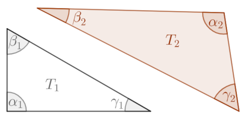
Answer: Since we talked about Banach spaces and linear algebra, some examples here have survived from those stories, so maybe some of the others may also be more "or-iginal." I will explain the essence of the two ideas with the image on the left and the application for the abo-ve example of mixture, and further to the model of the cosmos, perhaps another time. The sum of angles n-sided polygon is (n - 2)⋅180° in degrees, or (n - 2)⋅π in radians, and here the cases are considered only for n = 3.

1. Two triangles are similar iff they have equal angles. Thus, triangles T₁ and T₂ in the figure up on the left are not similar, because the angles of the first are α₁ = 90°, β₁ = 60°, γ₁ = 30°, while the angles of the second are α₂ = 100°, β₂ = 55°, and γ₂ = 25°, so we can talk about a “similarity coefficient” as a real number from 0 to 1.

Let's first define the "dissimilarity coefficient" using metrics like this. We ord-er the angles of the triangles by size and add up the three absolute differences of two by two (arbitrary) triangles and divide that sum by 180° if it is in degre-es, and when we work in radians, we divide it by π, as a measure of the distan-ce between them. For example, these in the picture have a dissimilarity coeffi-cient:

ρ(T₁, T₂) = (|α₁ - α₂| + |β₁ - β₂| + |γ₁ - γ₂|)/180° = 20/180 = 1/9.

It is easy to see that this definition satisfies the axioms of the metric and is si-milar to the well-known L₁. From it, we define the “similarity coefficient” as:

ς(T₁, T₂) = 1 - ρ(T₁, T₂) = 8/9 ≈ 0.889.

A seemingly unusual method of measuring the similarity of geometric figures, but in fact it is similar to face identification algorithms, such as the similarity of abstract theories of maybe tomorrows and who knows what else.

2. Another way to define the "amount of similarity" of two triangles would be by using linear operators or processes. The idea is to consider close phenome-na as those that pass more easily into each other or that would be separated by a shorter transformation process. Thus, in the case of the angles of triangles of non-increasing 3-term sequences (α_i ≥ β_i ≥ γ_i):

x₁ = (α₁, β₁, γ₁),   x₂ = (α₂, β₂, γ₂),

we notice various linear operators and their associated matrices A = (a_ij) of type 3×3. Let us consider the vector mappings Ax₁ = x₂, and let us limit ourselves to stochastic matrices. An example of such, for the triangles in the figure, is:

\[ \begin{pmatrix} 1 & 1/12 & 1/6 \\ 0 & 11/12 & 0 \\ 0 & 0 & 5/6 \end{pmatrix} \begin{pmatrix} 90^\circ \\ 60^\circ \\ 30^\circ \end{pmatrix} = \begin{pmatrix} 100^\circ \\ 55^\circ \\ 25^\circ \end{pmatrix}, \]

for the triangles from the previous image. We will call the determinant of the matrix, given det(A) = 55/72 ≈ 0.764, the "amount of similarity." To obtain a unique "amount," we must have a unique procedure for determining these st-ochastic matrices.

3. Proposition. If A is a stochastic matrix, and the elements of the sequence x are three angles of any triangle, then y = Ax is also a sequence of three angl-es of some triangle.

Proof: The members of the stochastic matrix are non-negative numbers that are the sums of 1 of the column elements, and the sum of the angles of the tr-iangle is 180° (π radians). Hence:

∥y∥₁ = |η₁| + |η₂| + |η₃| =
= (a₁₁ξ₁ + a₁₂ξ₂ + a₁₃ξ₃) + (a₂₁ξ₁ + a₂₂ξ₂ + a₂₃ξ₃) + (a₃₁ξ₁ + a₃₂ξ₂ + a₃₃ξ₃)
= (a₁₁ + a₂₁ + a₃₁)ξ₁ + (a₁₂ + a₂₂ + a₃₂)ξ₂ + (a₁₃ + a₂₃ + a₃₃)ξ₃
= 1⋅ξ₁ + 1⋅ξ₂ + 1⋅ξ₃ = ∥x∥₁

so if the first 3-term sequence x = (ξ₁, ξ₂, ξ₃) has a sum of 180°, the second 3-term sequence y = (η₁, η₂, η₃) will also have it. Sufficient for the definition of some triangle. ∎

For the sake of brevity, I use the notation 1-norm (Manhattan norm), which is one of the important ones in probability spaces. I assume that the angles of th-ese triangles are positive real numbers (the angles are not oriented), so I only write the absolute values ​​of the series terms at the beginning of the proof. This is convenient for the comfort of the algorithm for finding a unique stochastic mapping matrix of our angles, for which let's look at another example.

4. For angles x = (90°, 60°, 30°) and y = (80°, 70°, 30°) the corresponding co-py (Ax = y) will be:

\[ \begin{pmatrix} 8/9 & 0 & 0 \\ 1/9 & 1 & 0 \\ 0 & 0 & 1 \end{pmatrix} \begin{pmatrix} 90^\circ \\ 60^\circ \\ 30^\circ \end{pmatrix} = \begin{pmatrix} 80^\circ \\ 70^\circ \\ 30^\circ \end{pmatrix}, \quad \det(A) = 8/9. \]

For given angles x = (ξ₁, ξ₂, ξ₃) and y = (η₁, η₂, η₃) in three steps we find some stochastic matrix A : x → y starting from the identity matrix I of the third ord-er. In short, we proceed column by column, cut off the excesses when they ex-ist, and transfer them along the rows of the matrix from top to bottom. That's a separate story for another occasion.

Similarity II » srb

Question: You didn't finish that "other way" of defining (Similarity, 2) for wh-at you called the "amount of similarity" of polygons. Can you clarify that a li-ttle bit, at least using the example of triangles?

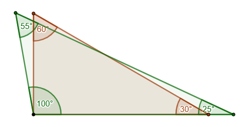
Answer: Okay, let's say we have triangles with non-increasing angles:

x = (ξ₁, ξ₂, ξ₃),   y = (η₁, η₂, η₃),

sums up to 180°, or π radians. The image on the right shows the two triangles from the image in the previous answer, to make it easier to see how similar they are. You can testify that ξ₁ = 90°, ξ₂ = 60°, ξ₃ = 30° and η₁ = 100°, η₂ = 55°, η₃ = 25°. Importantly, both are non-increasing se-quences, and then we look for the stochastic matrix A = (a_μν) of the third order.

1. The method of determining the linear operator, matrix A : x → y, is as foll-ows. By increasing the column (rows) of the matrix, indices are i, j ∈ {1, 2, 3}, we find the first pair ξ_i ≤ η_i and the second pair ξ_j > η_j. If there is no second pair, when all the angles of the first triangle are less than or equal to the corr-esponding ones (the angles are of non-increasing order), then their angles are equal and the similarity is complete. The matrix is ​​unitary (A = I) and its det-erminant is one (det A = 1), so we will say that the "similarity amount" of such two triangles is 1.

However, things get more interesting when we have a pair of angles, index i, where the first of the angles is not larger than the second, and the second pair of indices j where the first angle from x is larger than the corresponding one from y. Here it helps to notice the symmetry, so after finding the matrix for the case i = 1 and j = 2, we know how to apply it to other combinations. But more on that later. The following cases are detailed, starting from a third-order identity matrix and separating these situations.

2. When the first angle of the original is less than or equal to the copy, ξ₁ ≤ η₁, then the first column of the original unitary I matrix is ​​not changed. When the next pair is in the same order, ξ₂ ≤ η₂, then the second column is not changed either. The third column is thus forced. We calculate Ax = y, so:

ξ₁ + a₁₃⋅ξ₃ = η₁,     ξ₂ + a₂₃⋅ξ₃ = η₂,     a₃₃⋅ξ₃ = η₃

and it is assumed that a₁₃ + a₂₃ + a₃₃ = 1. Hence:

a₁₃ = (η₁ - ξ₁)/ξ₃,     a₂₃ = (η₂ - ξ₂)/ξ₃,     a₃₃ = η₃/η₃,

so the matrix is:

\[ A = \begin{pmatrix} 1 & 0 & \frac{\eta_1 - \xi_1}{\xi_3} \\ 0 & 1 & \frac{\eta_2 - \xi_2}{\xi_3} \\ 0 & 0 & \frac{\eta_3}{\xi_3} \end{pmatrix}, \quad \det(A) = \frac{\eta_3}{\xi_3}, \]

because ξ₁ ≤ η₁, then ξ₂ ≤ η₂, so ξ₃ > η₃. For example:

\[ \begin{pmatrix} 1 & 0 & 1/3 \\ 0 & 1 & 1/6 \\ 0 & 0 & 1/2 \end{pmatrix} \begin{pmatrix} 90^\circ \\ 60^\circ \\ 30^\circ \end{pmatrix} = \begin{pmatrix} 100^\circ \\ 65^\circ \\ 15^\circ \end{pmatrix}, \quad \det(A) = \frac12, \]

because 90° ≤ 100°, then 60° ≤ 55°, so 30° > 15°.

3. When the first and third angles of a pair are less than or equal to each other, then the second angle is greater, because the sum of the angles is 180°. In sho-rt, ξ₁ ≤ η₁ so ξ₂ > η₂ because ξ₃ ≤ η₃. Now we do not change the first and third columns (of the I matrix), and we calculate the second:

ξ₁ + a₁₂⋅ξ₂ = η₁,     a₂₂⋅ξ₂ = η₂     a₃₂⋅ξ₂ + ξ₃ = η₃.

Hence the stochastic matrix:

\[ A = \begin{pmatrix} 1 & \frac{\eta_1 - \xi_1}{\xi_2} & 0 \\ 0 & \frac{\eta_2}{\xi_2} & 0 \\ 0 & \frac{\eta_3 - \xi_3}{\xi_2} & 1 \end{pmatrix}, \quad \det{A} = \frac{\eta_2}{\xi_2}, \]

cases ξ₁ ≤ η₁, ξ₂ > η₂, ξ₃ ≤ η₃. For example:

\[ \begin{pmatrix} 1 & 1/60 & 0 \\ 0 & 59/60 & 0 \\ 0 & 0 & 1 \end{pmatrix} \begin{pmatrix} 90^\circ \\ 60^\circ \\ 30^\circ \end{pmatrix} = \begin{pmatrix} 91^\circ \\ 59^\circ \\ 30^\circ \end{pmatrix}, \quad \det(A) = \frac{59}{60}, \]

is that case, 90° ≤ 91°, 60° > 59°, 30° ≤ 30°. The similarity is great, det(A) ≈ 1.

4. When ξ₁ > η₁, and ξ₂ ≤ η₂ and ξ₃ ≤ η₃, then we shift the excess unit of the initial matrix from its first column down, with the measure a₁₁ξ₁ = η₁ and arrange it so that a₁₁ + a₂₁ + a₃₁ = 1, according to those that are missing. Therefore, we do not change either the second or third column (the initial matrix), and we recalculate the first:

a₁₁⋅ξ₁ = η₁     a₂₁⋅ξ₁ + ξ₂ = η₂,     a₃₁⋅ξ₁ + ξ₃ = η₃.

This results in the required matrix:

\[ A = \begin{pmatrix} \frac{\eta_1}{\xi_1} & 0 & 0 \\ \frac{\eta_2 - \xi_2}{\xi_1} & 1 & 0 \\ \frac{\eta_3 - \xi_3}{\xi_1} & 0 & 1 \end{pmatrix}, \quad \det(A) = \frac{\eta_1}{\xi_1}, \]

because ξ₁ > η₁, but ξ₂ ≤ η₂, and ξ₃ ≤ η₃. Such are the following examples:

\[ \begin{pmatrix} 8/9 & 0 & 0 \\ 0 & 1 & 0 \\ 1/9 & 0 & 1 \end{pmatrix} \begin{pmatrix} 90^\circ \\ 60^\circ \\ 30^\circ \end{pmatrix} = \begin{pmatrix} 80^\circ \\ 60^\circ \\ 40^\circ \end{pmatrix}, \quad \det(A) = 8/9, \]

because 90° > 80°, but 60° ≤ 60°, as well as 55° ≤ 60°. Also:

\[ \begin{pmatrix} 8/9 & 0 & 0 \\ 1/18 & 1 & 0 \\ 1/18 & 0 & 1 \end{pmatrix} \begin{pmatrix} 90^\circ \\ 55^\circ \\ 35^\circ \end{pmatrix} = \begin{pmatrix} 80^\circ \\ 60^\circ \\ 40^\circ \end{pmatrix}, \quad \det(A) = 8/9, \]

because 90° > 80°, but 55° ≤ 60°, as well as 35° ≤ < 40°.

5. When ξ₁ > η₁ and ξ₂ > η₂, then ξ₃ < η₃. We do not change the third column of the initial matrix I, but we truncate the units of the first and second to divi-de the excesses by the lower component of their columns. This follows:

a₁₁⋅ξ₁ = η₁,     a₂₂⋅ξ₂ = η₂,
a₁₁ + a₃₁ = 1,     a₂₂ + a₃₂ = 1,
a₃₁ = (ξ₁ - η₁)/ξ₁,     a₃₂ = (ξ₂ - η₂)/ξ₂,

and hence the transformation matrix:

\[ A = \begin{pmatrix} \frac{\eta_1}{\xi_1} & 0 & 0 \\ 0 & \frac{\eta_2}{\xi_2} & 0 \\ \frac{\xi_1 - \eta_1}{\xi_1} & \frac{\xi_2 - \eta_2}{\xi_2} & 1 \end{pmatrix}, \quad \det(A) = \frac{\eta_1}{\xi_1}\frac{\eta_2}{\xi_2}. \]

So, since ξ₁ > η₁ and ξ₂ > η₂, then ξ₃ < η₃. For example:

\[ \begin{pmatrix} \frac{9}{10} & 0 & 0 \\ 0 & \frac{12}{13} & 0 \\ \frac{1}{10} & \frac{1}{13} & 1 \end{pmatrix} \begin{pmatrix} 100 \\ 65 \\ 15 \end{pmatrix} = \begin{pmatrix} 90 \\ 60 \\ 30 \end{pmatrix}, \quad \det(A) = \frac{9}{10}\frac{12}{13}. \]

So, since 100° > 90° and 65° > 60°, so 15° < 30°.

6. If ξ₁ > η₁, but ξ₂ < η₂ because ξ₃ > η₃. The second column of the original matrix is ​​not changed, and the units of the first and third are truncated to transfer the excesses to the components of their columns. We calculate again, now from:

a₁₁⋅ξ₁ = η₁,     a₃₃⋅ξ₃ = η₃,
a₂₁ + a₃₁ = 1,     a₂₃ + a₃₃ = 1,
a₂₁ = (ξ₁ - η₂)/ξ₁,     a₂₃ = (ξ₃ - η₃)/ξ₃,

the matrix follows:

\[ A = \begin{pmatrix} \frac{\eta_1}{\xi_1} & 0 & 0 \\ \frac{\xi_1 - \eta_1}{\xi_1} & 1 & \frac{\xi_3 - \eta_3}{\xi_3} \\ 0 & 0 & \frac{\eta_3}{\xi_3} \end{pmatrix}, \quad \det(A) = \frac{\eta_1}{\xi_1}\frac{\eta_3}{\xi_3}, \]

which satisfies the given conditions ξ₁ > η₁, so ξ₂ < η₂ because ξ₃ > η₃. For example:

\[ \begin{pmatrix} \frac{9}{10} & 0 & 0 \\ \frac{1}{10} & 1 & \frac14 \\ 0 & 0 & \frac34 \end{pmatrix} \begin{pmatrix} 100 \\ 40 \\ 40 \end{pmatrix} = \begin{pmatrix} 90 \\ 60 \\ 30 \end{pmatrix}, \quad \det(A) = \frac{9}{10}\frac34, \]

satisfying the given conditions 100° > 90°, so 40° < 60° because of 40° > 30°.

7. When ξ₁ ≤ η₁, but ξ₂ ≥ η₂ and ξ₃ ≥ η₃ then we do not change the first colu-mn of the initial matrix, but we reduce the units in the second and third so that a₂₂⋅ξ₂ = η₂ and a₃₃⋅ξ₃ = η₃. This is the case ξ₁ + ξ₂ ≤ η₁ + η₂ and the last one is left. Then it goes a₂₁ = (ξ₂ - η₂)/ξ₂ without changing the bottom field (a₂₃ remains zero). And the third column is forced, a₁₃ = (ξ₃ - η₃)/ξ₃, so the matrix is:

\[ A = \begin{pmatrix} 1 & \frac{\xi_2 - \eta_2}{\xi_2} & \frac{\xi_3 - \eta_3}{\xi_3} \\ 0 & \frac{\eta_2}{\xi_2} & 0 \\ 0 & 0 & \frac{\eta_3}{\xi_3} \end{pmatrix}, \quad \det(A) = \frac{\eta_2}{\xi_2}\frac{\eta_3}{\xi_3}, \]

because ξ₁ ≤ η₁ while ξ₂ > η₂ and ξ₃ > η₃. I gave an example of this (Similarity 2), but here's another extreme one:

\[ \begin{pmatrix} 1 & 1/61 & 0 \\ 0 & 60/61 & 0 \\ 0 & 0 & 1 \end{pmatrix} \begin{pmatrix} 90^\circ \\ 61^\circ \\ 29^\circ \end{pmatrix} = \begin{pmatrix} 91^\circ \\ 60^\circ \\ 29^\circ \end{pmatrix}, \quad \det(A) = \frac{60}{61}, \]

because 90° ≤ 91° and 29° ≥ 29°. These triangles are very similar.

8. Note that the inequality ξ₃ > η₃ can be changed to ξ₃ ≥ η₃ and then, as in case (7), we obtain case (3), i.e., convert smaller-larger-larger into smaller-larger-smaller. However, the resulting matrix A is unique by this procedure, which presents a method suitable for estimating the “similarity distance” based on the determinant of the process A. It is unusual, because the “amount of similarity” is measured by the volume spanned by the operator vectors, which is det(A). This can only be discussed further.

Triads II » srb

Question: Can you write me the code for "similarity amount" and descriptions of how to use it?

Answer: The code is simple and I already have it in several variants. And you can easily get them by fo-llowing the steps in the attachment (Similarity II). One of the versions is here, written in Python 3.11.

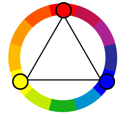
The program can be used to assess the similarity of various triads, fr-om fire triplet (substance, heat, ox-ygen), or music three-tones (funda-mental tone, third and fifth), Newt-on's palette (RYB) or digital (RGB) or similar color schemes, then che-mical triads (Döbereiner's), etc.

1. For example, it is known that the combination of red, which is coded by (255, 0, 0), green (0, 255, 0) and blue (0, 0, 255) light in the formation of a certain color (Color Codes) in a computer is created as a mixture (α, β, γ), where each of these three "angles" is an integer from 0 to 255. Thus, the so-called chocolate color x = (210, 105, 30) and sandy brown y = (244, 164, 96).

If we call the aforementioned program with these parameters, triads(x, y, 2), three are printed to the screen. Two are input arrays; now the norms ∥x'∥₁ = ∥y'∥₁ = 180. So x' = (109.565, 54.783, 15.652) and y' = (87.143, 58.571, 34.286) rounded to three decimal places. Then, the matrix and determinant were also rounded:

\[ A(x,y) = \begin{pmatrix} 0.795 & 0 & 0 \\ 0.035 & 1 & 0 \\ 0.170 & 0 & 1 \end{pmatrix}, \quad \det A(x,y) = 0.795 \]

The value of this determinant (0.795) is the "similarity" of the triangles with angles (109°, 55°, 16°) and (87°, 59°, 34°) rounded to whole numbers. If we calculate this directly (Similarity II, 4), we get:

a₁₁ = 87.143/109.565 ≈ 0.795,
a₁₂ = (58.571 - 54.783)/109.565 ≈ 0.035,
a₁₃ = (34.286 - 15.652)/109.565 ≈ 0.170,
det(A) ≈ 0.795,

and the rest are the coefficients of the identity matrix. As we can see, the results correspond to the accuracy taken here to the third decimal place.

2. The feature of this estimation is that it evaluates a variation of a single color but does not say anything about the type of that color. Thus, the choice of the mixture z = (96, 164, 244), otherwise blue, paired with x will result in the sa-me matrix A as the previous y, brown. However, the code variant, for example, "a, det = triads(x, z, 4)", which will not sort the input strings, will give a new matrix and determinant:

\[ A(x,z) = \begin{pmatrix} 0.313 & 0 & 0 \\ 0.035 & 1 & 0 \\ 0.652 & 0 & 1 \end{pmatrix}, \quad \det A(x,z) = 0.313 \]

A reduced determinant speaks of a lesser "similarity" of mixtures, a pair of the same shades but colors from different groups. They're both brown, here brown and blue.

3. The next "oddity" of this triad estimate is the difference in mapping:

A(x, y) : x → y,     A(y, x) : y → x,
A(x, y) ≠ A(y, x),     A(x, y) ≠ A^-1(x, y).

The matrix A is stochastic and otherwise maps probabilities, and as such it do-es not have an inverse stochastic matrix (which does not mean that it does not have an inverse matrix). For example:

\[ A(x,y) = \begin{pmatrix} 1 & 1/61 & 0 \\ 0 & 60/61 & 0 \\ 0 & 0 & 1 \end{pmatrix} \begin{pmatrix} 90^\circ \\ 61^\circ \\ 29^\circ \end{pmatrix} = \begin{pmatrix} 91^\circ \\ 60^\circ \\ 29^\circ \end{pmatrix}, \quad \det(A) = \frac{60}{61}, \] \[ A(y,x) = \begin{pmatrix} 1 & 1/91 & 0 \\ 0 & 90/91 & 0 \\ 0 & 0 & 1 \end{pmatrix} \begin{pmatrix} 91^\circ \\ 60^\circ \\ 29^\circ \end{pmatrix} = \begin{pmatrix} 90^\circ \\ 61^\circ \\ 29^\circ \end{pmatrix}, \quad \det(A) = \frac{90}{91}, \] \[ A^{-1}(x,y) = \begin{pmatrix} 1 & -1/61 & 0 \\ 0 & 60/61 & 0 \\ 0 & 0 & 1 \end{pmatrix}, \quad \det(A^{-1}) = \frac{61}{60}. \]

The determinant det A(x, y) = 60/61 is the "similarity amount" of the triangles x and y, a number from 0 to 1; the larger the greater the similarity. The inverse is also called the amount, A(y, x) = 90/91 because both matrices are stochast-ic; they copy the angles of an arbitrary triangle into the angles of some triangle (Similarity, 3. Proposition), and therefore they do not have an inverse that wo-uld be stochastic because the minimalism principle applies to random events.

The processes of the state lead to more probable, or less informative, states; therefore, the reverse flow is not spontaneous; it is not stochastic. Spontaneity of this kind implies the possibility of choice, and various mappings then requ-ire us to choose A as the basic one from this set (f : x → y).

4. Similarity measured by stochastic processes starts from the right to options, and with the law of large numbers, it reaches analogous certainties. In short, by linking the process, by transferring a copy to a new copy in the same way, everything that such a stochastic chain copies in steps is getting closer and closer to one and the same copy, which is actually the inherent state of that “copying machine.”

Thus the previous matrix A(x, y), whose general form dictates the stated co-ndition ξ₁ ≤ η₁, so ξ₂ ≥ η₂ and ξ₃ ≥ η₃ (Similarity II, 7), has the characteristic equations:

\[ Av = \begin{pmatrix} 1 & \frac{\xi_2 - \eta_2}{\xi_2} & \frac{\xi_3 - \eta_3}{\xi_3} \\ 0 & \frac{\eta_2}{\xi_2} & 0 \\ 0 & 0 & \frac{\eta_3}{\xi_3} \end{pmatrix} \begin{pmatrix} \frac{180^\circ\xi_2}{2\xi_2 - \eta_2} \\ \frac{180^\circ(\xi_2 - \eta_2)}{2\xi_2 - \eta_2} \\ 0 \end{pmatrix} = \begin{pmatrix} \frac{180^\circ\xi_2}{2\xi_2 - \eta_2} \\ \frac{180^\circ(\xi_2 - \eta_2)}{2\xi_2 - \eta_2} \\ 0 \end{pmatrix} = v, \] \[ \begin{pmatrix} 1 & 1/61 & 0 \\ 0 & 60/61 & 0 \\ 0 & 0 & 1 \end{pmatrix} \begin{pmatrix} \frac{180^\circ\cdot 61}{62} \\ \frac{180^\circ}{62} \\ 0 \end{pmatrix} = \begin{pmatrix} \frac{180^\circ\cdot 61}{62} \\ \frac{180^\circ}{62} \\ 0 \end{pmatrix} \approx \begin{pmatrix} 177.097^\circ \\ 2.903^\circ \\ 0 \end{pmatrix}. \]

This is the solution of the matrix equation Av = λv, for the eigenvalue λ = 1, which is the case for every stochastic matrix. Such a matrix will copy the tri-angle with angles (91°, 60°, 29°) into the triangle with angles (90°, 61°, 29°), the latter into some third, the third again further and further, converging towards the triangle with angles (178°, 3°, 0), rounded to integers. It is act-ually a series of classes of all similar triangles of various side sizes, but given angles.

Opposites III » srb

Question: Can we use the orientation of the angles in "triads"?

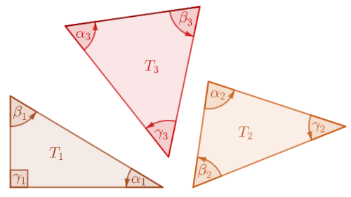
Answer: Yes, "similarity" estimates can also take into account the orie-ntation of the triangle, but then th-ey come with new interesting featu-res. First of all, with the use of neg-ative values ​​in new, more conveni-ent "stochastic" matrices.

The news is quite a bit, and I have to add a few clarifications to this story. In the picture on the right are three triangles, T₁, T₂ and T₃, angles:

T₁ :     α₁ = 60°,   β₁ = 30°,   γ₁ = 90°,
T₂ :     α₂ = 40°,   β₂ = 80°,   γ₂ = 60°,
T₃ :     α₃ = 60°,   β₁ = 70°,   γ₃ = 50°.

The first two are positive orientations (counterclockwise), but the third is the opposite (the angles rotate clockwise). Note that triangles of the same orienta-tion can be sorted (non-increasing sequence of angles) with a simple rotation in the plane. Thus, we sort the first sequence with one right shift and the ang-les of the second with two shifts, while this is not possible with the third:

T₁ :   (α₁, β₁, γ₁) → (γ₁, α₁, β₁),
T₂ :   (α₂, β₂, γ₂) → (β₂, γ₂, α₂),
T₃ :   (α₃, β₃, γ₃) → (β₃, α₃, γ₃).

Then, let us recall that all identical transformations (that do not change the distances between points) of geometry can be reduced to rotations (Action of Information, 255. Rotations). When we have an opposite isometry (the image and the original are triangles of opposite orientation), then we perform the rotation through a new dimension of space. We pick up the triangle T₃, turn it over, and put it back on the table, so we will have all three triangles of the same orientation on the table.

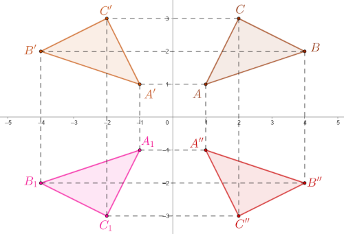
The image on the left shows the triangle ΔABC in the rectangular Cartesian system Oxy. It is axi-symmetrically mapped about the vertical axis into the triangle ΔA'B'C', and about the horizontal axis into the triangle ΔA''B''C''. Both images are triangles with the opposite orientation to the original. However, if one of these two imag-es were to be axially mapped again, we would get a copy of the copy ΔA₁B₁C₁, or ΔABC, again with the same orientation as the original. Compare this to the multiplication of negative numbers given by a positive number.

More precisely, an axial mapping (general reflection) changes the sign of the other axis. Applied twice, it changes their product (the composition of the ma-pping) to the initial sign. In this way, we can also understand negative "proba-bilities," i.e., "stochastic" matrices with negative coefficients. The lesson is th-is: a triangle changes orientation when its angles change sign.

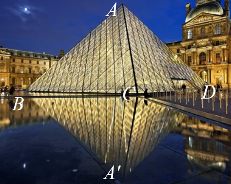
The image on the right shows the Louvre Glass Pyramid ABCD and its reflection on the surface A'BCD with four mirrored triangles:

ΔABC → ΔA'BC,
ΔACD → ΔA'CD,
ΔADB → ΔA'DB,
ΔBCD → ΔBCD

its sides. Each one changes the orientation of the vertices; that is, each of the reflections changes the orientation of the angles.

Therefore, if we change the signs of the angles of a triangle with reversed orie-ntation:

T₃ = (α₃, β₃, γ₃)   →   T'₃ = -(α₃, β₃, γ₃),

so that each of the angles changes sign:

α₃ → -α₃,     β₃ → -β₃,     γ₃ → -γ₃,

The triangle will change the orientation of its vertices. Then sorting its angles will be possible by shearing, one to the right:

T₃ :   (60°, 70°, 50°) → (-60°, -70°, -50°) → (-50°, -60°, -70°).

The angles are now negative but in decreasing (non-ascending) order. The sa-me would be achieved if the reflective surface for the pyramid were not the gr-ound, but rather, say, the facade of a building as a mirror.

It makes no difference if we introduce a fourth dimension as time. The angle ∠BAC is positive if we consider that the arm AB rotates on the surface of the triangle ΔABC with the fixed point A counterclockwise. The opposite flow of time, viewed on a film played backwards, would show such a rotation in the clockwise direction, so the angle ∠CAB = -∠BAC.

Applied to stochastic matrices, its negative coefficients will be negative proba-bilities and will represent the inverse of the time course of the process. Then the principle of minimalism should be reversed into the principle of maxima-lism, or something similar. The phenomenon is theoretical, therefore univer-sal, and one should abstract the lengths of the sides of similar triangles, which can be different for the same “amounts of similarity.” For example, different masses can have the same volumes.

And that would be it, as far as the orientation of the angles in the “triads” is concerned. Can we now move on to the more serious part of this topic?

Stochastic II » srb

Question: So, can you tell me something "serious" about these pseudo-stocha-stic processes? I got this (Opposites III); maybe I'll get that too.

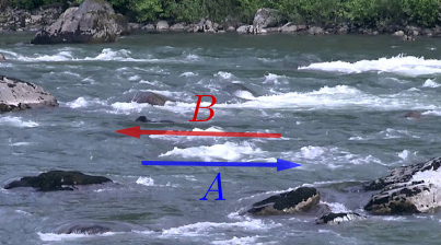
Answer: A pseudo-stochastic matr-ix is ​​a square matrix with a column sum of each of the absolute values ​​of elements from [-1, 1].

1. It is like this:

\[ B = \begin{pmatrix} \frac65 & \frac{8}{15} & -\frac45 \\ -1 & \frac73 & -1 \\ \frac45 & -\frac{28}{15} & \frac{14}{5} \end{pmatrix}, \]

because the sum of each column is 1, however, B is not a true stochastic matrix because it also has negative coefficients. The inverse matrix of this one is:

\[ A = B^{-1} = \begin{pmatrix} 0.7 & 0 & 0.2 \\ 0.3 & 0.6 & 0.3 \\ 0 & 0.4 & 0.5 \end{pmatrix}, \]

so A^-1 = B. While A represents processes that go "downstream" (an allusion to the image on the left), because they follow the principle of minimalism, the pr-ocesses B are "upstream." However, not every pseudo-stochastic matrix is ​​the inverse of a stochastic one.

2. The following two pseudo-stochastic matrices are mutually inverse:

\[ \begin{pmatrix} 0.7 & 0.8 & 0 \\ -0.3 & 0.6 & 1 \\ 0.6 & -0.4 & 0 \end{pmatrix} \begin{pmatrix} 0.526 & 0 & 1.053 \\ 0.789 & 0 & -0.921 \\ -0.316 & 1 & 0.868 \end{pmatrix} = \begin{pmatrix} 1 & 0 & 0 \\ 0 & 1 & 0 \\ 0 & 0 & 1 \end{pmatrix}, \]

rounded to three decimal places. Both represent "unnatural" processes with disrupted spontaneity, for example, by the action of forces that would come from outside into their closed system of conservation, the amount of inform-ation.

3. Let us recall that nature is built on information characterized by uncertain-ty. Therefore, natural phenomena spontaneously flow towards less informati-ve ones, because more probable outcomes are more frequent, and therefore behave in such a way that uncertainty is a repulsive force. Hence the Maupe-rtuis principle of least action, that the product of mass, velocity, and distance traveled is constant, mvs = const, because bodies do not want to communicate (interact). Not wanting what is precisely that makes them.

This leads, on the one hand, to the law of conservation of energy, that the sum of kinetic and potential is constant, and on the other, that their difference is constant. And then to a slow gradual sliding from one state to another, passing through dense positions between them (Adaptation II). Changes are inevitable in such a world, so what is most likely in the first step is not the same in the next. Everything adapts to its environment and in each subsequent step it sees it as slightly different, but different enough to make the jump in movement and process in general less likely.

4. Therefore, phenomena are "unnatural," I say, if they are disturbed by a distraction from outside some system that surrounds them, which will also produce "natural" changes in its own way, depending on the unexpectedness added to them. They are then again in some closed system.

Algebraically, this means that the product of (pseudo) stochastic processes, or their matrices, is again a (pseudo) stochastic process. Namely:

\[ \sum_j c_{ij} = \sum_j\sum_k a_{ik}b_{kj} = \sum_k a_{ik}(\sum_j b_{kj}) = \sum_k a_{ik} = 1, \]

which means that the product of (pseudo) stochastic matrices (a_ij) and (b_ij) will give such a (pseudo or ordinary) stochastic matrix (c_ij). The consequence of this is that the product of a (pseudo) stochastic matrix and a vector of a gi-ven constant sum of terms gives vectors with the same constant sum. This was just the introduction to "seriousness". I mean, there's a sequel if you're intere-sted.

Polygon » srb

Question: How do you calculate the area of ​​a polygon in a coordinate system?

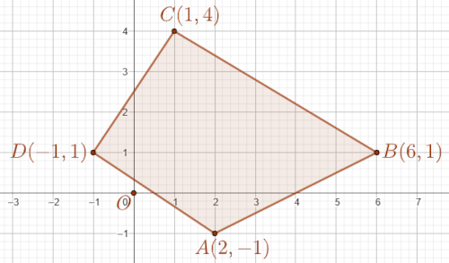
Answer: If you have a chance to see my script “Trougao” (2014), then I recommend commutators. It was once an unnoticed elementary me-thod of calculating the areas of po-lygons, whether convex or concave, in any case.

For example, in the figure on the right is a convex quadrilateral ABCD whose vertices are A(2, -1), B(6, 1), C(1, 4), and D(-1, 1), in addition to the origin O(0, 0) in the Cartesian rectangular coordinate system. We use the following point notations: T(T_x, T_y) and the commutator notation [P, Q] = P_xQ_y - Q_xP_y. The area of ​​this quadrila-teral is twice:

2Π(ABCD) = [A, B] + [B, C] + [C, D] + [D, A] =
= (A_xB_y - B_xA_y) + (B_xC_y - C_xB_y) + (C_xD_y - D_xC_y) + (D_xA_y - A_xD_y)
= (2⋅1 - 6⋅(-1)) + (6⋅4 - 1⋅1) + (1⋅1 - (-1)⋅4) + ((-1)⋅(-1) - 2⋅1)
= 8 + 23 + 5 - 1 = 35,

so the area of ​​the given quadrilateral Π(ABCD) = 35/2. I'll explain why.

1. Example (heuristic). Note that the quadrilateral ABCD consists of two tri-angles, area Π(ABD) + Π(BCD), common base BD = 7, with heights 2 and 3. Therefore, the double area of ​​the quadrilateral is:

Π(ABCD) = Π(ABD) + Π(BCD) = 7⋅2 + 7⋅3 = 35,

and that is the same result as before. ∎

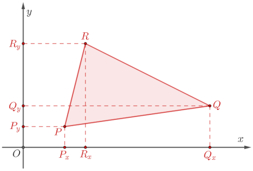
2. Now that we have verified that the above result is correct, let's no-tice in the image on the left that the triangle PQR has an area consisting of three trapezoids, the sum of R_x-Q_xQR and P_xR_xRP from which we need to subtract P_xQ_xQP:

(Q_y + R_y)⋅(Q_x - R_x)/2 +
(R_y + P_y)⋅(R_x - P_x)/2 -
(Q_y + P_y)⋅(Q_x - P_x)/2 =

(Q_yQ_x - Q_yR_x + R_yQ_x - R_yR_x)/2 +
(R_yR_x - R_yP_x + P_yR_x - P_yP_x)/2 -
(Q_yQ_x - Q_yP_x + P_yQ_x - P_yP_x)/2 =

= (P_xQ_y - Q_xP_y)/2 + (Q_xR_y - R_xQ_y)/2 + (R_xP_y - P_xR_y)/2
= [P, Q]/2 + [Q, R]/2 + [R, P]/2 ,

2Π(PQR) = [P, Q] + [Q, R] + [R, P].

Therefore, the double area of ​​a triangle is obtained by adding the commutato-rs in the direction of the triangle, analogous to the quadrilateral above.

3. Using this, we add two triangles into a quadrilateral of area:

2Π(ABCD) = 2Π(ABC) + 2Π(CDA) =
= ([A, B] + [B, C] + [C, A]) + ([C, D] + [D, A] + [A, C])
= [A, B] + [B, C] + [C, D] + [D, A],

because [C, A] = -[A, C]. And that is the result from the introduction. Starting from one vertex, we can divide each polygon into triangles using diagonals, and by stringing these commutators together in the same orientation of the triangles, we can obtain the polygon's area.

4. According to Kepler's second law (Conics), a motion from the Sun to a pla-net sweeps out equal areas in equal times. If the Sun is at the origin of such a coordinate system, in infinitesimal times this motion will sweep out equal ar-eas to the orbit and will make equal commutators along it. This can be trans-ferred to probability spaces, for example, Chebyshev's inequality.

Due to its connection with the force of probability, commutators are an impor-tant part of this information theory, especially as external information (In and Out), a feature of this theory. The internal information is the perceptual scalar product of the vectors. When the third vertex of the triangle is the origin O, in general, the internal and external information are (θ = ∠u,v):

I_← = u⋅v = u_xv_x + u_yv_y = uv cos θ,
I_→ = [u, v] = u_xv_y - v_xu_y = uv sin θ.

The combination of the two is complex information (i² = -1):

I = I_← + iI_→ = uv(cos θ + i sin θ) = uv e^iθ.

This is easily generalized to multiple dimensions in which the vertices of the same polygon can be found.

Polygon II » srb

Question: Can the formulas for mapping the angles of a triangle (Similarity II) be applied to polygons?

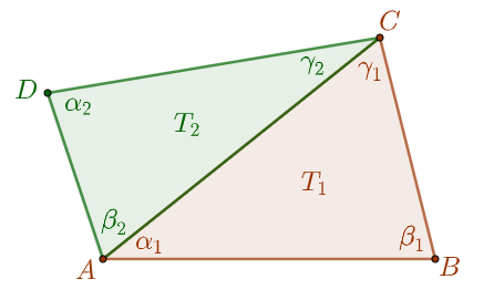
Answer: Of course they can. Then we have (n-2)⋅180° for the angle sum of the n-th angle. In the figure on the left we see how by adding a new vertex (D) the previous angle sum (α₁ + β₁ + γ₁ = 180° of the triangle T₁) increases by 180°. In the figure, the quadrilateral ABCD is the union of two triangles T₁ ∪ T₂, with a total of 360° interior degrees. We do not have to repeat the entire procedure of finding the angle mapping matrix of two such triangles, but we will notice the analogy.

1. When we map n-angles into each other with the matrix A = (a_ij), the marked angles of the first x = (ξ₁, ξ₂, ..., ξ_n)^⊤ and the second y = (η₁, η₂, ..., η_n)^⊤, so th-at for some j = 1, 2, ..., n we have the angle of the first larger than the second, ξ_j > η_j, and all others are less than or equal to, ξ_k ≤ η_k for k ≠ j, will be the jth column of the matrix:

\[ a_{.j} = \left(\frac{\eta_1-\xi_1}{\xi_j}, ..., \frac{\eta_{j-1}-\xi_{j-1}}{\xi_j}, \frac{\eta_j}{\xi_j}, \frac{\eta_{j+1}}{\xi_j}, ..., \frac{\eta_n - \xi_n}{\xi_j}\right)^\top, \]

where η_j/ξ_j is the diagonal element of the matrix. The other columns are iden-tity matrices. For example (Ax = y, n = 4, j = 2):

\[ \begin{pmatrix} 1 & (\eta_1 - \xi_1)/\xi_2 & 0 & 0 \\ 0 & \eta_2/\xi_2 & 0 & 0 \\ 0 & (\eta_3 - \xi_3)/\xi_2 & 1 & 0 \\ 0 & (\eta_4 - \xi_4)/\xi_2 & 0 & 1 \end{pmatrix} \begin{pmatrix} \xi_1 \\ \xi_2 \\ \xi_3 \\\xi_4 \end{pmatrix} = \begin{pmatrix} \eta_1 \\ \eta_2 \\ \eta_3 \\ \eta_4 \end{pmatrix}, \quad \det A = \eta_2/\xi_2, \]

when ξ₁ ≤ η₁, ξ₂ > η₂, ξ₃ ≤ η₃, ξ₄ ≤ η₄. Such is the case:

\[ \begin{pmatrix} 1 & 5/120 & 0 & 0 \\ 0 & 110/120 & 0 & 0 \\ 0 & 5/120 & 1 & 0 \\ 0 & 0 & 0 & 1 \end{pmatrix} \begin{pmatrix} 90^\circ \\ 120^\circ \\ 80^\circ \\70^\circ \end{pmatrix} = \begin{pmatrix} 95^\circ \\ 110^\circ \\ 85^\circ \\ 70^\circ \end{pmatrix}, \quad \det A = 11/12, \]

because it is 90° ≤ 95°, 120° > 110°, 80° ≤ 85°, 70° ≤ 70°.

2. When there are m ∈ {2, ..., n-1} angles from the first n-th angle x that are larger than the corresponding ones of the second y, then each such j-th dia-gonal a_jj = η_j/ξ_j, and all other elements of that row are zero. The remaining columns are of the identity matrix, and in the rows of the columns of the me-ntioned diagonals there are fractions a_ij = (ξ_i - η_i)/mξ_j. For example (Ax = y, n = 4, m = 2, j₁ = 2 and j₂ = 3):

\[ \begin{pmatrix} 1 & (\eta_1 - \xi_1)/2\xi_2 & (\eta_1 - \xi_1)/2\xi_3 & 0 \\ 0 & \eta_2/\xi_2 & 0 & 0 \\ 0 & 0 & \eta_3/\xi_3 & 0 \\ 0 & (\eta_4 - \xi_4)/2\xi_2 & (\eta_4 - \xi_4)/2\xi_3 & 1 \end{pmatrix} \begin{pmatrix} \xi_1 \\ \xi_2 \\ \xi_3 \\\xi_4 \end{pmatrix} = \begin{pmatrix} \eta_1 \\ \eta_2 \\ \eta_3 \\ \eta_4 \end{pmatrix}, \quad \det A = \frac{\eta_2}{\xi_2}\frac{\eta_3}{\xi_3}, \]

када је ξ₁ ≤ η₁, ξ₂ > η₂, ξ₃ > η₃, ξ₄ ≤ η₄. Такво је пресликавање:

\[ \begin{pmatrix} 1 & 1/24 & 1/22 & 0 \\ 0 & 22/24 & 0 & 0 \\ 0 & 0 & 20/22 & 0 \\ 0 & 1/24 & 1/22 & 1 \end{pmatrix} \begin{pmatrix} 70° \\ 120° \\ 110° \\60° \end{pmatrix} = \begin{pmatrix} 80° \\ 110° \\ 100° \\ 70° \end{pmatrix}, \quad \det A = \frac{22}{24}\frac{20}{22}, \]

јер је 70° ≤ 80°, 120° > 110°, 110° > 100°, 60° ≤ 70°.

3. The program (Python 3.13.3) for this calculation is shown in the image.

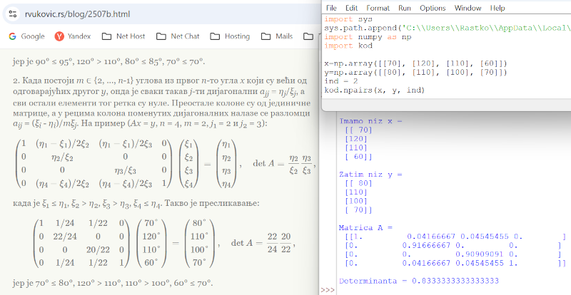
The code is in the attachment "A pair of n-th angles" here on the Codes page. The amount of similarity is the determinant at the end of that report.

4. Recall that the "freedom" S = I⋅H is equal to the product of the "intelligen-ce" I (ability) and the "hierarchy" H (constraints), and that it is maximal when these two factors are equal (Completion). It is not the same, but analogous to this, that a homogeneous probability distribution (Extremes) achieves maxi-mal information. Also, here we have the greatest similarity if the mapping determinant is one; otherwise, it is smaller.

It is something like the largest volume of a body with the smallest surface ar-ea, such as a ball or a cube among parallelepipeds. The determinant of the nth order is the generalized n-dim "volume" of its column vectors, and this is larg-est when it is traversed by mutually perpendicular (unit) vectors. Then the si-milarity of the polygons is total because their corresponding angles are exactly equal.

5. For the "amount of similarity," det(A), the lengths of the sides do not matter if they are proportional (Thales' theorem). Since it is largest (det A = 1) when we have complete similarity of triangles, this determinant is like a snowplow that captures and transfers the original angles to the copied ones.

In this way, mapping by operators in general can be understood as more or le-ss directing the copied to the copied by "capturing." If the reception and tran-smission are not compatible, then only partial transfers occur, so |det A| < 1.

Usage » srb

Question: Where can this "quantity of similarity" method be applied?

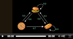
Answer: This is a typical question and always reminds me of a joke that a woman should never be as-ked about her age, a man about his salary, and a mathematician about where it is used. However, I believe that there is nothing more useful than a good theory.

1. For example, the video on the right explains Markov chains and their application, and "similarity quantities" can be applied there as well.

A customer will come in and ask for a hamburger, pizza, or hotdog. Let's say it was one of three occurrences: A, B, or C. If it was A (a hamburger was purcha-sed), the chance that it was preceded by A is P_AA = 0.2, that it was then B is P_AB = 0.3, and that it was C is P_AC = 0.5. If B (buying a pizza) just happened, there is no chance that it was B before, nor that it was C, and P_BA = 0.6 is the probability of A before. Before C (buying a hotdog), the chance that the previ-ous customer had the same order is P_CC = 0.5, as is the probability P_CA = 0.2 that it was A, and P_CB = 0.7 that it was B.

2. Briefly, we can write this situation in matrix form (x' = Mx):

\[ \begin{pmatrix} a' \\ b' \\ c' \end{pmatrix} = \begin{pmatrix} P_{AA} & P_{AB} & P_{AC} \\ P_{BA} & P_{BB} & P_{BC} \\ P_{CA} & P_{CB} & P_{CC} \end{pmatrix} \begin{pmatrix} a \\ b \\ c \end{pmatrix}. \]

This is not only a reviewed record but also an opportunity for matrix multi-plication. This is made possible by the conditional probability formulas (In-formation Coupling), because:

a' = P_AA a + P_AB b + P_AC c.

When a, b and c are the probabilities that at a given moment the exact oppo-rtunity for A, B, or C (a hamburger, pizza, or hotdog buyer) has arisen, then a' appears as the new probability that the next one will be A. The same applies to the others.

3. However, the equality is also true if the input vector numbers (x), and the-refore the output (x' = Mx), are, say, the total turnover of events (items sold) in certain periods. When we wait for a flow of 180 occurrences (all sales), after which a uniform occurrence of three possibilities, x = (60, 60, 60), occurs, th-en this matrix equality (x' = Mx) gives the following distribution:

\[ \begin{pmatrix} 60 \\ 36 \\ 84 \end{pmatrix} = \begin{pmatrix} 0.2 & 0.3 & 0.5 \\ 0.6 & 0 & 0 \\ 0.2 & 0.7 & 0.5 \end{pmatrix} \begin{pmatrix} 60 \\ 60 \\ 60 \end{pmatrix}, \quad \det(M) = 0.12. \]

The determinant 0.12 of this matrix is ​​not zero, which means that from the ou-tput (x') it is possible to calculate the input (x = M^-1x'), but this is not the mat-rix (Triads II) with which we would estimate the "amount of similarity" of the strings. It would be:

\[ A(x, x') = \begin{pmatrix} 1 & 0 & 0 \\ 0 & 0.6 & 0 \\ 0 & 0.4 & 1 \end{pmatrix}, \quad \det(A) = 0.6. \]

We see, this matrix is ​​more efficient than the previous one, det(A) = 2⋅det(M). It finds a shorter process, A : x → x', lower cost, i.e., less interference (channel noise); we would say a shorter path and a better estimate of the "similarity amount" of the two sequences. The example also confirms the ambiguity of such mappings.

4. Both are stochastic matrices, and such matrices always have a unit for the eigenvalue. We then find the eigenvectors from:

Mu = u,     Av = v,

\[ u = \begin{pmatrix} 0,352 \\ 0,211 \\ 0,437 \end{pmatrix}, \quad v = \begin{pmatrix} p \\ 0 \\ 1-p \end{pmatrix}, \]

with an arbitrary parameter p. These are unit L₁ norms so that they can be interpreted as probability distributions. If we multiply them by 180, we get:

\[ U = \begin{pmatrix} 63 \\ 38 \\ 79 \end{pmatrix}, \quad V = \begin{pmatrix} 180p \\ 0 \\ 180q \end{pmatrix}, \]

where p + q = 1. This means that sales under M will stabilize at 63, 38, and 79 items in portions of 180 sold, while under model A it would have different sta-bilizations depending on the choice of p, with no pizza being sold at all.

5. Planning is another application of this. Conditional probabilities, for exam-ple, can be used to guide the selection or design of places for the sale of items, and then stable sales can be learned from the eigenvectors. This saves on sub-sequent statistics (from trial and error) and speeds up successful prediction by working with more reliable means. The waste is decreasing.

Limitations » srb

Question: Where are the limitations of stochastic operators?

Answer: The same sums of terms in each column of the matrix generate their constraints. I'll talk about that first, and perhaps most important-ly.

1. Commutator:

K = [A, B] = AB - BA

of the stochastic matrices A and B is not reversible. This is a property of all pseudo-stochastic matrices, i.e., in general, matrices of equal sum columns (Stochastic II). The product of such matrices is again of this type, so the difference K is the zero-sum column, and these are then vectors that do not span space, i.e., the determinant det(K), i.e., the volume of the space they span, is zero. Since det(K) = 0, K is not rever-sible.

2. Since they are not reversible, the operators whose matrices define the above commutators (K) have no past, do not represent durations or any "reality". Commutators of (pseudo) stochastic matrices represent fictions. They are an additional way of such representations, in addition to the null space (Fictiti-ous). However, it is precisely in such examples that we see how fictions can become reality.

3. Example. Let us show that a pseudo-stochastic matrix can have a stocha-stic matrix as its inverse.

Solution: Such are the following matrix and its inverse:

\[ A = \begin{pmatrix} -1 & 4 \\ 3 & -2 \end{pmatrix}, \quad A^{-1} = \begin{pmatrix} 0.2 & 0.4 \\ 0.3 & 0.1 \end{pmatrix}. \]

It is easy to see that the product of these two is an identity matrix, AA^-1 = I. ∎

4. Example. Let us show that (pseudo) stochastic matrices are not commuta-tive.

Solution: The following two matrices are such.

\[ AB = \begin{pmatrix} -1 & 4 \\ 3 & -2 \end{pmatrix} \begin{pmatrix} 2 & -3 \\ -5 & 0 \end{pmatrix} = \begin{pmatrix} -22 & 3 \\ 16 & -9 \end{pmatrix}, \quad \det(AB) = 150, \] \[ BA = \begin{pmatrix} 2 & -3 \\ -5 & 0 \end{pmatrix} \begin{pmatrix} -1 & 4 \\ 3 & -2 \end{pmatrix} = \begin{pmatrix} -11 & 14 \\ 5 & -20 \end{pmatrix}, \quad \det(BA) = 150. \]

The column sums of the first matrix (A) are 2, the column sums of the second (B) are -3, and the column sum of each of these products is -6. The determina-nt of the product is equal to the product of the determinants, here 150, so each of the four has an inverse matrix. However, the difference of their products is not reversible:

\[ K = AB - BA = \begin{pmatrix} -11& -11 \\ 11 & 11 \end{pmatrix}, \quad \det(K) = 0. \]

These are pseudo-stochastic matrices, so their special type of stochastic (non-negative elements of unit sum columns) have the same properties. ∎

5. Finally, we have an example (Momentum II) of a commutator:

\[ [\hat{x}, \hat{p}] = \hat{x}\hat{p} - \hat{p}\hat{x} = i\hbar\hat{I}, \]

which has an inverse matrix which is not made up of (pseudo) stochastic ma-trices but rather matrices of position and momentum operators whose column sums are not equal. These are infinite matrices because the position distances as well as the magnitudes of the momentum have no upper bounds.

Due to the reversible commutator, in short, a coupling of position and mome-ntum arises that has a past, has duration, and is a fundamental property of re-ality. Stochastic operators, however, do not have this possibility. Their coupli-ngs of this kind are limited to fictions.

Fake Metric » srb

Question: Are these "quantities" we are discussing metrics of some spaces?

Answer: No, in the mathematical sense the "quantities" in question are not metrics of a space. Or ra-ther, they are not norms of some metric spaces, because then we imply the following.

1. Definition (Norm). A vector space (X, Φ) is normed if there exists a non-negative function defined ∀x ∈ X, which we call the norm of X and denote by ∥x∥, such that:

1. ∥0∥ = 0 and ∥x∥ > 0 for x ≠ 0, positivity,
2. ∥λx∥ = |λ|∥x∥ for each λ ∈ Φ, homogeneity,
3. ∥x + y∥ ≤ ∥x∥ + ∥y∥, triangle inequality.

Although the above "quantities" do not have these three properties, they are still usable.

2. If we simply added numbers, as in the columns of pseudo-stochastic matri-ces, for example, it would be ∥(1, -1)∥ = 1 - 1 = 0, even though the summands are not zero and the first axiom (positivity) of the norm would not be fulfilled. The third (triangle inequality) is also not fulfilled, because it should be:

∥(2, 1)∥ ≤ ∥(2, -1)∥ + ∥(-1, 1)∥,
2 + 1 ≤ (2 - 1) + (-1 + 1),
3 ≤ 1 + 0,

which is clearly not true. For example, for L₁ this would be true, because:

∥(2, 1)∥₁ ≤ ∥(2, -1)∥₁ + ∥(-1, 1)∥₁,
|2| + |1| ≤ (|2| + |- 1|) + (|-1| + |1|),
3 ≤ 3 + 2.

Also, the first condition for L₁ is true since from ∥(a, b)∥₁ = 0, or |a| + |b| = 0, it follows that a = b = 0, whatever the numbers a and b are, real or complex.

3. Nor is the property of maintaining the constancy of the sum of columns after matrix multiplication tenable, when we consider the "sum" as a norm. Let's look at this using the example of the most common, so-called Euclidean norm, L₂:

\[ \|x\|_2 = \sqrt{|\xi_1|^2 + ... + |\xi_n|^2}, \quad x = (\xi_1, ..., \xi_n). \]

We work with 2-dim matrices of unit (L₂) norm (AB = C₁):

\[ \begin{pmatrix} 3/5 & 12/13 \\ 4/5 & 5/13 \end{pmatrix} \begin{pmatrix} 7/25 & 15/17 \\ 24/25 & 8/17 \end{pmatrix} = \begin{pmatrix} 1.054 & 0.964 \\ 0.593 & 0.887 \end{pmatrix}, \]

rounded to three decimal places. The root of the sum of squares (L₂) in the first column of the result is 1.210 but the same norm of the second column is 1.310. Multiplication does not leave the norms of the column vectors equal.

4. Matrix multiplication is not commutative here either (BA = C₂ ≠ C₁):

\[ \begin{pmatrix} 7/25 & 15/17 \\ 24/25 & 8/17 \end{pmatrix} \begin{pmatrix} 3/5 & 12/13 \\ 4/5 & 5/13 \end{pmatrix} = \begin{pmatrix} 0.874 & 0.598 \\ 0.952 & 1.067 \end{pmatrix}, \]

so it makes sense to check the commutator (K = C₁ - C₂):

\[ K = [A, B] = \begin{pmatrix} 0.180 & 0.366 \\ -0.359 & -0.180 \end{pmatrix}, \quad \det(K) = 0.099 \]

rounded to three decimal places. Therefore, the matrix equation Kx = 0 has only a trivial solution. The Null space of the matrix K has no vectors other than zero x = 0.

July II 2025 (Original ≽)