February 2026 (Original ≽)

Boiled frog » srb

Question: The gradual shearing of the light polarizer (Evasion, 4) reminds me a lot of the boiled frog method?

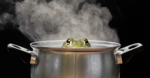
Answer: You're right, that's a good observation. This famous allegory of the "boiled frog" is about a frog that will escape from suddenly bo-iling water, but when placed in cold water that is slowly heated, it will stay there and be cooked. Or about the general and our failure to notice danger until it is too late. The ques-tion is, does this have any applicat-ion in correlations?

1. Correlation is the quotient of covariance, the measure of the relationship be-tween X and Y, the pairs of random variables, and the variances, standard de-viations (average deviations from the mean):

$$ \kappa_{x,y} = \text{corr}(X,Y) = \frac{\text{cov}(X,Y)}{\sigma_x\sigma_y} = \frac{\sum_{i=1}^n(x_i - \mu_x)(y_i - \mu_y)}{\sqrt{\sum_{j=1}^n(x_j-\mu_x)^2\sum_{k=1}^n(y_k-\mu_y)^2}}. $$

The arithmetic mean of a sequence is the number μ_x = (x₁ + x₂ + ... + x_n)/n, of the n-tuple, and the sequence of its differences are the numbers Δx_i = x_i - μ_x. The mean value of the square of these differences is the variance, that is the number σ_x² = (Δx₁² + Δx₂² + ... + Δx_n²)/n. And the root of the variance is the standard deviation of σ_x. The covariance is the mean of the dot product of differences, cov(x, y) = (Δx₁ Δy₁ + Δx₂ Δy₂ + ... + Δx_n Δy_n)/n.

2. For example, x = (22, 35, 29, 34, 39, 42, 45), y = (12, 24, 17, 23, 29, 33, 36) are 7-term arrays of mean values:

μ_x = (22 + 35 + 29 + 34 + 39 + 42 + 45)/7 ≈ 35.143
μ_y = (12 + 24 + 17 + 23 + 29 + 33 + 36)/7 ≈ 24.857

Based on them, we form differences, series of deviations of the members of the series from its mean value, here roughly (for μ_x = 35 and μ_y = 25):

Δx = X - μ_x = (-13, 0, -6, -1, 4, 7, 10)
Δy = Y - μ_y = (-13, -1, -8, -2, 4, 8, 11)

The sums of squares of the (roughly) found sequences give the variances:

$$ \sigma^2_x = \frac{1}{n}\sum_j^n (x_k - \mu_x)^2 = (169 + 0 + 36 + 1 + 16 + 49 + 100)/7 = 53.00 $$ $$ \sigma^2_y = \frac{1}{n}\sum_k^n (y_k - \mu_y)^2 = (169 + 1 + 64 + 4 + 16 + 64 + 121)/7 \approx 62.71 $$

and the roots of these are the standard deviations:

σ_x ≈ 7.28     σ_y ≈ 7.92

We calculate the covariance as the mean of the dot product:

cov(x, y) = (169 + 0 + 48 + 2 + 16 + 56 + 110)/7 ≈ 57.29

This is the numerator of the correlation, and in the denominator are two stan-dard deviations:

$$ \text{corr}(x,y) = \frac{\text{cov}(x,y)}{\sigma_x\sigma_y} \approx \frac{57.29}{7.28\cdot 7.92} \approx 0.994 $$

Otherwise, correlation is a real number from -1 to +1, where +1 is in the case of a perfect direct, increasing linear relationship, and −1 is in the case of a perfect inverse, or opposite, decreasing linear relationship (anticorrelation).

3. For example, in Python (3.11.0), we calculate the same thing like this:

import numpy as np

def korelacija(X,Y):
    if len(X)==len(Y):
        Sum_xy = sum((X-X.mean())*(Y-Y.mean()))
        Sum_x_squared = sum((X-X.mean())**2)
        Sum_y_squared = sum((Y-Y.mean())**2)       
        corr = Sum_xy / np.sqrt(Sum_x_squared * Sum_y_squared)
    return corr
            
# Define the dataset
x = np.array([22, 35, 29, 34, 39, 42, 45])
y = np.array([12, 24, 17, 23, 29, 33, 36])
z = np.array([10, 20, 30, 40, 50, 60, 70])

xy = korelacija(x,y)
yz = korelacija(y,z)
zx = korelacija(z,x)

print('corr(x,y):', xy)    
print('corr(y,z):', yz)
print('corr(z,x):', zx)

corr(x,y): 0.9943382674616695
corr(y,z): 0.9201519915209659
corr(z,x): 0.9126423311754243

I have listed three strings x, y and z with three correlations listed at the end 0.99, 0.92 and 0.91, to make it easier to understand what the product of two correlations of three variables means and that such a, say corr(x,y) ⋅ corr(y,z), is not always smaller/larger than the third corr(z,x). However, the correlation of such a pair is limited by the product of the other two: corr(x,z) ≥ 2 corr(x,y) corr(y,z) - 1.

4. We note that seemingly different random sequences can have very high correlations. This can be confusing, so the limit of the first two, such as 2⋅0.994⋅0.920 - 1 ≈ 0.829, is a fairly loose correlation, close to 0.829. In a series of such connected pairs x, y, z, ..., if we look only at the pairs of adjacent ones and their correlations corr(x, y), corr(y, z), corr(z, u), ..., it may seem to us that the situation does not change and that we do not notice the dangers until it is too late, or let's say that we have a frog placed in cold water that is slowly warming up and that remains there in ignorance until it is cooked. This is not just an illusion, but a rationally explicable phenomenon, because a seri-es of such powers (even the number 0.99) decreases exponentially rapidly.

Restriction » srb

Question: I know that correlation is not transitive, but are there any restricti-ons on κ_ac correlations, if the κ_ab and ρ_bc correlations are known?

Answer: Yes, correlation is indeed not transitive. For example, with independent variables X and Y let:

A = X,   B = X + Y,   C = Y.

In the general case, from the values

κ_ac = corr(a, b),   κ_bc = corr(b, c)

we can't have κ_ac = corr(a, c) with absolute precision, but there are some rou-gh estimates. You can read about this in the book Information of Perception (2016) in the section "3.6 Stereometry of statistics", pp. 91-96. If someone had asked me this question back then, I would have listed the answers there, whi-ch I will now add. For the sake of clarity, I will repeat part of that content.

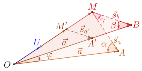
1. Somewhere, two n-tuples of random variables A(a₁, a₂, ..., a_n) and A'(a'₁, a'₂, ..., a'_n) are given with an n-tuple U(1, 1, ..., 1). They form three vectors $\vec{a}$, $\vec{a}'$ and $\vec{u}$ of some n-dim vector space. With a single origin (O), these vectors in pairs span the planes shown in the figure above right, with the angle between the given random vectors ∠(AOA') = φ.

In this case, the projection of point A onto direction OU is point M into which some point B of direction OA' is also projected, while point A' is projected into M' of the same direction OU. Then we have angles ∠(MAO) = α, ∠(MBO) = β and ∠(AMB) = γ. The joins, sticks are vectors:

$$ \vec{s}_a = \overrightarrow{MA}, \quad \vec{s}_{a'} = \overrightarrow{M'A'}, \quad \vec{s}_b = \overrightarrow{MB} $$

perpendicular to the vector $\vec{u}$. The proof that the triangle OAM is right-angled, where ∠M = 90°, is given in the aforementioned book (Theorem 3.6.1.), and starts from the points:

$$ \overrightarrow{OM} = \mu_a\,\vec{u}, \quad \overrightarrow{OM'} = \mu_{a'}\,\vec{u}, $$

where μ_a = (a₁, a₂, ..., a_n)/n and μ_a' = (a'₁, a'₂, ..., a'_n)/n are the arithmetic means of the given random sequences.

2. From the (same) image we read and calculate:

$$ \overrightarrow{OM} + \overrightarrow{MA} = \overrightarrow{OA}, \quad \overrightarrow{OM'} + \overrightarrow{M'A'} = \overrightarrow{OA'}, $$ $$ \vec{s}_a = \vec{a} - \mu_a\,\vec{u}, \quad \vec{s}_{a'} = \vec{a}' - \mu_{a'}\,\vec{u}. $$

This means that the components of the joins Δa_i = a_i - μ_a and Δa'_j = a'_j - μ_a' respectively, with indices i, j = 1, 2, ..., n. The scalar product of such joins is:

$$ \vec{s}_a\cdot\vec{s}_{a'} = \Delta a_1\,\Delta a'_1 + \Delta a_2\,\Delta a'_2 + ... + \Delta a_n\,\Delta a'_n = \sum_{k=1}^n \Delta a_i\,\Delta a'_i, $$ $$ \text{cov}(a, a') = \vec{s}_a\cdot\vec{s}_{a'}/n. $$

Their intensities are:

$$ \|\vec{s}_a\|^2 = \sum_{j=1}^n (\Delta a_j)^2, \quad \|\vec{s}_{a'}\|^2 = \sum_{k=1}^n (\Delta a'_k)^2, $$ $$ \sigma^2_a = \|\vec{s}_a\|^2/n, \quad \sigma^2_{a'} = \|\vec{s}_{a'}\|^2/n. $$

So, the correlation of the given random sequences is:

$$ \kappa_{a,a'} = \frac{\vec{s}_a\cdot\vec{s}_{a'}}{\|\vec{s}_a\|\,\|\vec{s}_{a'}\|} = \cos\gamma, $$

which we get after truncating the fraction by n and considering that the vector is divided by the intensity of unit length. The scalar product of vectors is the product of their intensities and the cosine of the angle between them.

3. When we have three random sequences, n-tuples of numbers, we have the vectors:

$$ \vec{a} = (a_1, a_2, ..., a_n), \quad \vec{a}' = (a'_1, a'_2, ..., a'_n), \quad \vec{a}'' = (a''_1, a''_2, ..., a''_n), $$

to whose pairs we can apply the previous consideration. We get:

$$ \kappa_{a,a'} = \cos\gamma, \quad \kappa_{a',a''} = \cos\gamma', \quad \kappa_{a'',a} = \cos\gamma''. $$

These are correlations of pairs of given vectors, they are not angles between vectors, but between $\vec{s}_a$, $\vec{s}_{a'}$ and $\vec{s}_{a''}$ perpendicular to $\vec{u} = (1, 1, ..., 1)$:

$$ \gamma = \angle(\vec{s}_a,\vec{s}_{a'}), \quad \gamma' = \angle(\vec{s}_a',\vec{s}_{a''}), \quad \gamma'' = \angle(\vec{s}_{a''},\vec{s}_{a}). $$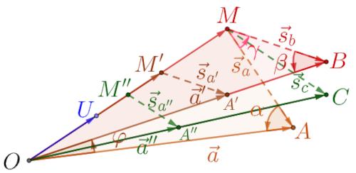

In the figure on the left, the n-tuple $\vec{a}''$ is added in green to the previous two. It is projected into OM'', that is, the sequence (μ_a'', μ_a'', ..., μ_a''), where μ_a'' is also the arithmetic mean of the elements of the given vector. By homothety, this conne-ction is extended to the point M into the connection $\vec{s}_c || \vec{s}_{a''}$. From the figure, it can be seen that the angle γ could be from the interval from the difference to the sum of the other two angles, from |γ' - γ''| to |γ' + γ''|, i.e.

$$ \cos(\gamma' + \gamma'') \le \cos\gamma \le \cos(\gamma' - \gamma''), $$ $$ \cos\gamma'\cos\gamma'' - \sin\gamma'\sin\gamma'' \le \cos\gamma \le \cos\gamma'\cos\gamma'' - \sin\gamma'\sin\gamma'', $$ $$ \kappa_{bc}\kappa_{ca} - \sqrt{1 - \kappa^2_{bc}}\sqrt{1 - \kappa^2_{ca}} \le \kappa_{ab} \le \kappa_{bc}\kappa_{ca} + \sqrt{1 - \kappa^2_{bc}}\sqrt{1 - \kappa^2_{ca}}, $$

because √(1 - κ_bc²) = √(1 - cos²γ') = sin γ' and equally √(1 - κ_ca²) = sin γ''. And, more precisely, on the left side of these inequalities one should choose greater than -1 or the value of the given expression, and on the right side less than +1 and given. This is one of the relations of the aforementioned constraints.

4. Let's look at the same previous finding in a slightly different way. The cos-ine of any angle is not greater than one and, third, the cosine of the sum is known:

cos(γ' + γ'') = cos γ' cos γ'' - sin γ' sin γ'',     cos(γ' + γ'') ≤ cos γ ≤ 1.

Hence cos γ' cos γ'' - 1 ≤ -sin γ' sin γ'', so 2 cos γ' cos γ'' - 1 ≤ cos γ, that is:

$$ 2\kappa_{bc}\kappa_{ca} - 1 \le \kappa_{ab} $$

This is the inequality listed as a comment at the end of the item from the previous answer (Boiled frog, 3).

Intensity » srb

Question: How do we compare restrictions from "stereometry of statistics" to the polarization of light?

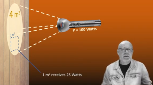
Answer: The projection of the leng-th A₀ onto the axis between which the angle θ is A = A₀ cos θ. On the other hand, a 100 W battery light (as in the picture on the left) proje-cted onto an area of ​​4 m² will give one quarter of that intensity per square meter, so I = I₀ cos²θ. This latter is known as Malus's law. Wh-at happens when light is polarized is a loss of intensity. We distinguish this from the mere decay of the amplitude of light and, in fact, this is what the Born's law measures.

1. When we project a plane with an angle (φ), the vertex of the angle and the points on the arms are not equally distant from their projections, so the resu-lting angle (γ) is larger than the original (φ ≤ γ). This is evident in the aforem-entioned images (from the previous answer). Because the angle between the joints, then $\angle(\vec{s}_a,\vec{s}_b) = \gamma$ is larger than the angles of the random sequences $\gamma \ge \alpha = \angle(\vec{a},\vec{a'})$, so the cosine of the projected angle is larger than the cosine of the projection (cos φ ≥ cos γ). That is why the scalar product is derived the-re via "stereometry of statistics", because the correlation is more accurate that way. By squaring the cosine of the larger angle, the error of the cosine of the smaller angle can be reduced.

2. Measurement in quantum mechanics is the finding of observables of an op-erator Q which are its eigenvectors v, such that they can solve the characteri-stic equation Qv = λv, where λ ∈ ℝ is an eigenvalue. These vectors v₁, v₂, ..., each with an associated eigenvalue λ₁, λ₂, ... form the basis of a quantum sy-stem, the vector space they span. Similar matrices (Q' ∼ Q with Q' = P^-1QP) have the same eigenvalues, not the same associated eigenvectors. Depending on the basis of the system in which we define a matrix, we obtain its different representations.

Such a matrix Q = (q_jk) represents a quantum system with the mapping Q: x → y, or written Qx = y, where the vectors from its space are:

x = (ξ₁, ξ₂, ...) = ξ₁ v₁ + ξ₂ v₂ + ...
y = (η₁, η₂, ...) = η₁ v₁ + η₂ v₂ + ...
η_j = q_j1ξ₁ + q_j2ξ₂ + ...,   j = 1, 2, ...

Such vectors are the states of a quantum system defined by the matrix Q. Wh-en we measure them, they are projected onto the axis (eigenvectors) by proba-bility, the first |ξ_k|², or the second |η_j|². The squares of the modulus of the complex numbers ξ_k, η_j ∈ ℂ are real numbers, and we can also understand them as the squares of the cosines of the angles of the vectors with respect to axes that are also positive numbers of sum one (as are probability distributi-ons). These squares of cosines, again, can also be understood as correlations. We most often find what is most likely, that is, what best correlates with the measurement conditions.

3. Three famous Pauli matrices (Bloch sphere):

$$ \sigma_x = \begin{pmatrix} 0 & 1 \\ 1 & 0 \end{pmatrix}, \quad \sigma_y = \begin{pmatrix} 0 & -i \\ i & 0 \end{pmatrix}, \quad \sigma_z = \begin{pmatrix} 1 & 0 \\ 0 & -1 \end{pmatrix} $$

can be viewed as a "vector" $\vec{\sigma} = (\sigma_x, \sigma_y, \sigma_z)$. Let us define the spin operator along the unit vector û as:

$$ \hat{S} = \frac{\hbar}{2}\,\vec{\sigma}\cdot\hat{u} = \frac{\hbar}{2}\,(\sigma_x a_x, \sigma_y a_y, \sigma_z a_z), $$ $$ \hat{S} \psi = \frac{\hbar}{2}\,\vec{\sigma}\cdot\hat{u}\,\binom{\psi_1}{\psi_2}. $$

When the spin of a particle is determined by the eigenstate, or vector ψ, of the Ŝ operator, then Ŝψ = λψ for λ ∈ ℝ. For example, if we measure the spin along the z-axis when û = (0, 0, 1), then $\vec{\sigma}\cdot\hat{u} = \sigma_z$, so for the equation Ŝ_z ψ = λψ, in detail:

$$ \frac{\hbar}{2}\begin{pmatrix} 1 & 0 \\ 0 & -1 \end{pmatrix} \begin{pmatrix} \psi_1 \\ \psi_2 \end{pmatrix} = \lambda\begin{pmatrix} \psi_1 \\ \psi_2 \end{pmatrix} $$

we find two solutions, eigenstates:

$$ \psi_+ = \binom{1}{0}, \quad \psi_- = \binom{0}{1}, $$

eigenvalues ​​λ₊ = ℏ/2 and λ_- = -ℏ/2.

Instead of Ŝ we write only the operator $\vec{\sigma}\cdot\hat{u}$, without Planck's constant, and then we have nicer eigenvalues ​​±1 for spin "up" and "down". In general, a particle in the û direction has a measured spin-up, when the eigenvalue is +1, and a spin-down if the eigenvalue is -1. The polarization of light is strongly correlated with this.

4. In the spherical coordinate system when the deviation from the z-axis is an angle θ, then with an arbitrary φ in the Oxy plane, we have û = (sin θ cos φ, sin θ sin φ, cos θ) and:

$$ \vec{\sigma}\cdot \hat{u}\, \psi = \lambda \psi, $$ $$ (\sigma_x\cos\theta\cos\varphi + \sigma_y\sin\theta\sin\varphi + \sigma_z\cos\theta)\psi = \lambda \psi, $$ $$ \begin{pmatrix} \cos\theta & \sin\theta\cos\varphi - i\sin\theta\sin\varphi \\ \sin\theta\cos\varphi + i\sin\theta\sin\varphi & -\cos\theta \end{pmatrix} \begin{pmatrix} \psi_1 \\ \psi_2 \end{pmatrix} = \lambda \begin{pmatrix} \psi_1 \\ \psi_2 \end{pmatrix}, $$ $$ \begin{pmatrix} \cos\theta & \sin\theta\, e^{-i\varphi} \\ \sin\theta\, e^{i\varphi} & -\cos\theta \end{pmatrix} \begin{pmatrix} \psi_1 \\ \psi_2 \end{pmatrix} = \lambda \begin{pmatrix} \psi_1 \\ \psi_2 \end{pmatrix}, $$

so again we find the eigenvalues ​​λ = ±1 with the corresponding eigenvectors ψ_±. For example, for φ = 0 and θ = 60° we have:

$$ \begin{pmatrix} \frac12 & \frac{\sqrt{3}}{2} \\ \frac{\sqrt{3}}{2} & -\frac12 \end{pmatrix} \begin{pmatrix} \frac{\sqrt{3}}{2} \\ \frac12 \end{pmatrix} = \begin{pmatrix} \frac{\sqrt{3}}{2} \\ \frac12 \end{pmatrix}, \quad \begin{pmatrix} \frac12 & \frac{\sqrt{3}}{2} \\ \frac{\sqrt{3}}{2} & -\frac12 \end{pmatrix} \begin{pmatrix} \frac12 \\ -\frac{\sqrt{3}}{2} \end{pmatrix} = -\begin{pmatrix} \frac12 \\ -\frac{\sqrt{3}}{2} \end{pmatrix}. $$

The eigenvalue λ of the operator $\vec{\sigma}\cdot \hat{u}$ is always +1 or -1, there is no third. This means that there is only "spin-up" or "spin-down", no third in passing particl-es through a magnet with respect to the north-south orientation of the magn-et. What we find in such experiments are the Expected value, $E[(\vec{\sigma}\cdot \hat{u})\,\psi]$, of the particle current intensity.

5. In the Stern-Gerlach experiment, after vertical selection, the initial silver atoms will have a current of cos²(θ/2) in the upward direction through the magnet's tilt, and sin²(θ/2) in the downward direction. The mean value of the spin-up redirected particles is the mean tilt, the angle θ/2, and the square of the cosine of the angle comes from Malus's law of intensities.

When the probability of turning up |ψ|² = p for the value of the variable λ = +1, and the probability of turning down |ψ|² = q for the variable λ = -1, then the expectation, or mean, is E[ψ] = (+1)p + (-1)q, where p + q = 1 and p, q ≥ 0. By Malus's law, this expectation is E[ψ] = cos²(θ/2) - sin²(θ/2) = cos θ. We have no contradiction in transferring the restriction method from the stere-ometry of statistics to the polarization of light, nor to spin deflections.

Expected » srb

Question: In statistics we have a theoretical expected value based on practical outcomes, and in quantum physics it turns out the other way around, the exp-ected value is practical and the possibilities are theoretical?

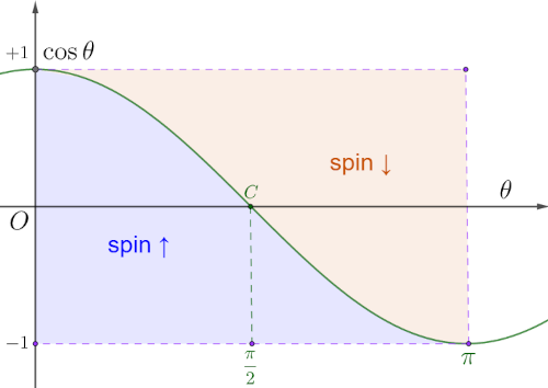
Answer: That's right, you're sharp. After measuring an electron, its previous trajectory is also created (Heisenberg, 1927), that is, only by opening the "box with the cat" is it defined whether this "cat" was alive or dead before. That's how things are in quantum physics. Not in the macro-world when the laws of large numbers conceal its coincidences.

1.When we randomly draw one of four equal balls labeled with numb-ers from the set X = {1, 2, 3, 4} in order, the expected value of a drawn is:

E[X] = ∑(number)×(probability) = (1 + 2 + 3 + 4)/4 = 2.5.

However, there is no such ball. In the macro-world, this result makes sense as the average value of the numbers of balls drawn after many draws.

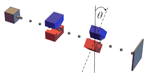
Experiment (Intensity, 5) on the left, behind a vertical north-south magnet, a beam of silver atom pa-rticles flows through a magnet til-ted by an angle θ relative to the first. We measure the angle in pl-anes perpendicular to the current. And the expectation is the opposite: the spin of silver atoms when they pass through the magnet can theoretically have many directions, but the mea-sured particle current is divided into only two streams, i.e. spin-up and spin-down (Bohm and Aharonov [Phys. Rev. 108, 1070 (1957)]). Only with the me-asurement is the previous state of the quantum particles defined.

In the picture, up right, according to the mentioned experiment, the mean va-lue (expectation) will be $\langle \vec{\sigma}\cdot\hat{a}\rangle = \cos\theta$ . This is also a correlation, a number from -1 to +1. Now, by using the brackets (from quantum mechanics) for the mean value, we emphasize a slightly different meaning of the same calculati-on, which is otherwise part of probability theory. The unit vector $\hat{u}$ of the ma-gnet's direction is now $\hat{a}$ , like Alice, because later we also need $\hat{b}$, like Boban.

In that figure is a cosine graph showing that the highest probability of spin-up will be for a particle jet with an angle θ = 0 of inclination of the unit vector $\hat{a}$ to the north-south axis of the magnet. This probability decreases with the cosine of the angle and with θ = π/2, when cos θ = 0, the spin-up and spin-down flow distributions become equal. For further angles θ ∈ (π/2, π) there would still theoretically be spin-up particles, just as there would be spin-down particles for angles θ ∈ (0, π/2).

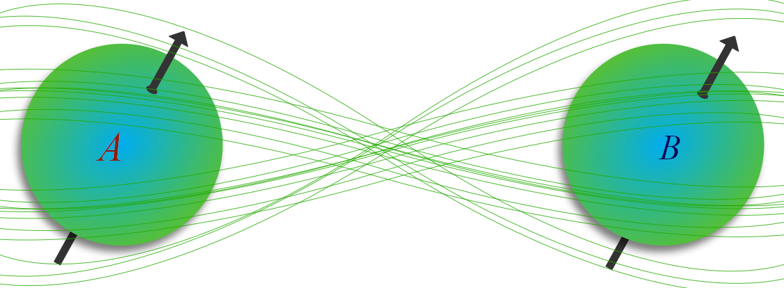
2. The third image, on the right, is the quantum entanglement (coup-ling) noticed by Alice and Boban. The arrows show the orientation of the magnets from the previous image and they do not have to be parallel, but at an angle θ, as in that Stern-Gerlach experiment. The first magnet (vertical) is now Alice, and the second (inclined) is Boban, but this is the (EPR paradox) from 1935.

Alice and Boban calculate the given singlet state, quantum entanglement, but from different coordinate systems. They each write their own, proper formula, in order:

$$ A: \quad \Psi(x_1,x_2) = \sum_{n=1}^\infty \psi_n(x_2)u_j(x_1) \quad \to \quad u_k(x_1), \quad \psi_k(x_2), $$ $$ B: \quad \Psi(x_1,x_2) = \sum_{s=1}^\infty \varphi_s(x_2)v_k(x_1) \quad \to \quad v_r(x_1), \quad \varphi_r(x_2). $$

When working with similar matrices of a given process, A and B calculate the same eigenvalues, with which the spin up/down is determined, but not the same eigenvectors. The arrows on the right show the first and second results of Alice and Boban from their points of view. The notations are from Einste-in's original paper (here), but not the interpretation in which we now see the correlation and the restriction described above.

The basic misunderstanding of this quantum entanglement comes from the simultaneity of events that Alice and Boban do not see as simultaneous. They see particles A and B in different places and at different times, while this singlet state is in itself simultaneous and acting on A means acting on B as well, which I wrote about before, so I won't go into it now. I add here that by measuring A, this state collapses from the superposition and withdraws the declaration of its part B as well. Collapses occur in such short times (at the atomic level) that we consider them to be zero. Realistically, it takes time for information from Bob to reach Alice, if they are very distant, so it is a specu-lative question how simultaneous these events really are for Alice.

3. Unlike classical correlation, the individual states of entangled particles are not predetermined. The particles exist in a superposition that defines them only when one of them is measured. The moment you measure one particle, the state of the other is instantly determined—even if it is light years away. This nonlocal behavior defies the usual logic of physics, or the understanding that it is a consequence of some hidden variables proposed by Einstein and his colleagues after the discovery of this paradox (1935). However, Bell's theorem (1964) proved that there are no such parameters, and then a series of physical experiments established the existence of this strange coupling.

Ordinary correlation can always be explained by shared information from the past. However, quantum entanglement does not have local correlations that follow classical probability, and this is confirmed by Bell's theorem and rela-ted experiments. This is the idea of ​​Bell's proof that there are no secret para-meters in quantum entanglement, which, when applied in this way, leads to a contradiction of the concept of classical correlation. On the other hand, it may also mean a request for an expansion of the understanding of "correlation".

4. The classical correlation κ(x, y) = corr(x, y) of the x = (ξ₁, ξ₂, ..., ξ_n) with the sequence y = {η₁, η₂, ..., η_n} is a real number from -1 to +1 obtained by calcula-ting:

$$ \kappa(x,y) = \frac{\sum_{i=1}^n (\Delta \xi_i\,\Delta \eta_i)}{\sqrt{\sum_{j=1}^n (\Delta \xi_i)^2}{\sqrt{\sum_{k=1}^n (\Delta \eta_k)^2}}} = \frac{\Delta x \cdot \Delta y}{\|\Delta x\| \|\Delta y\|}, $$

where the changes are Δξ_i = ξ_i - μ_x and Δη_i = η_i - μ_y for i = 1, 2, ..., n, and μ_x and μ_y are the means, or expectations, of the sequences x and y. In the nume-rator of the fraction on the right is the scalar product of the series of differen-ces, Δx⋅Δy, and in the denominator are the factors of the two intensities of those series of differences, ∥Δx∥ and ∥Δy∥. Therefore, the correlation is:

$$ \kappa(x,y) = \hat{x}\cdot\hat{y}, \quad \hat{x} = \frac{\Delta x}{\|\Delta x\|},\ \hat{y} = \frac{\Delta y}{\|\Delta y\|}. $$

It is the scalar product of normalized, therefore unit series of differences, i.e. vectors Δx = (ξ₁ - μ_x, ξ₂ - μ_x, ..., ξ_n - μ_x) and Δy = (η₁ - μ_y, η₂ - μ_y, ..., η_n - μ_y). One of its interpretations of this information theory is information perception. In other words, when quantum entanglement exists, there is no information transfer, or communication, or interaction between particles. When possible, this notation is easily translated into integral form.

Singlet » srb

Question: Explain to me the part (Expected, 2) next to the third image. What does it mean that Alice and Boban see a singlet with the same eigenvalues ​​of spin, but unequal eigenvectors u and v?

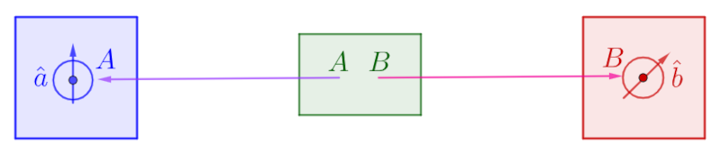
Answer: In linear algebra, similar matrices A and B represent the same linear mapping within some vector space, but given from two of its bases. Then there exists a matrix P such that A = P^-1BP, the eigenvalues ​​of these matrices are eq-ual sets, but the sets of their corresponding eigenvectors may be different.

In the figure above we see what happens when a single state, then called a sin-glet, is split into two parts by interpretation in different bases of the same qua-ntum space, that is, the eigenvectors that are spanned by the matrix interpre-tations of the given process. Noticing a new physical exposition of linear alge-bra, Einstein and his colleagues (1935) discovered quantum entanglement, considering this to be a consequence of either some hidden parameters, or the inadequacy of that algebra in quantum mechanics.

1. In particular, we consider the situation of two diverging particles, of total momentum zero and spin zero, which repel each other so that the momentum of the first is p, and the momentum of the second is -p. Whether integer or half-integer, the particles have spin-up (+1) and spin-down (-1), but it is not known which one belongs to which until there is an interaction. When they are in a superposition, the spin of each is not actually formed. The first particle is at position x₁, the second is translated to x₂.

The superposition collapses into a single outcome like a rolled die that results in a single number, i.e., a declaration into one of the eigenvectors but the only possible eigenvalues ​​that achieve an overall zero spin. For Alice, this is a coll-apse into the state u_k(x₁) when the other particle becomes φ_k(x₂), and for Boban, it is a collapse into the state v_r(x₁) when the other remains in φ_r(x₂).

2. Einstein's idea of ​​hidden parameters, which Bell denoted with the same symbol λ as eigenvalues ​​from which we need to distinguish them, is that we have $A(\hat{a}, \lambda) = \pm 1/2$ and $B(\hat{b}, \lambda) = \pm 1/2$. Bell's parameter λ can be any set of quantities (vectors, tensors, etc.), but simply let it be a scalar. So the assum-ption is that the result A of the measurement $\vec{\sigma}_1\cdot\hat{a}$ depends on the unit vector â of Alice's basis and the hidden parameters λ, while the result B of the measu-rement $\vec{\sigma}_2\cdot\hat{b}$ will depend on the unit vector of Boban's basis but the same hid-den parameters, without the influence â on B and vice versa.

Bell formulates this using a correlation:

$$ \kappa(\hat{a},\hat{b}) = \int A(\hat{a},\lambda)B(\hat{b},\lambda)\rho(\lambda)\,d\lambda $$

where ρ(λ) is the probability density of these observations. It is integrated ov-er all values ​​of the parameter λ. For example, when the unit vectors (from the image) are equal, so parallel and the angle θ = 0 between them, cos θ = 1, and:

$$ \kappa(\hat{a},\hat{a}) = \int (\pm)(\mp)\rho(\lambda)\,d\lambda = -1, $$

because the probability in all the possibilities is a certainty, ∫ ρ(λ) dλ = 1. When the unit vectors are opposite, the angle θ = π between them and the cosine -1, there will be such a correlation κ(â, -â) = 1. When the unit vectors are perpendicular, the polarization axes are perpendicular to each other and there is an equal chance that the spin will turn up or down, and there is no correlation, κ = 0.

Considering these and more complex examples, Bell found a contradiction which he (very sparingly and hard to read) published in his famous paper. You will find more detailed explanations, which I am abbreviating here, in more extensive quantum mechanics lectures, but they are not the point of this story as much as the limitations of known correlation and information perception (Expected, 4).

3. Let us note, by the way, that the above three (extreme) examples of correla-tion:

κ(↑, ↑) = -1,     κ(↑, →) = 0,     κ(↑, ↓) = +1,

can be explained by "hidden parameters". They coincide with the quantum ex-pectation $\langle \hat{a}, \hat{b}\rangle = \hat{a}\cdot\hat{b} = \cos\theta$ whose cosines are the values ​​of these three nu-mbers. Note that the case of a solitary particle can also be explained by a "hid-den parameter" which is the angle θ ∈ (0, π) of the spin deflection (imaginary orientation) before the measurement which results in only two values ​​+1 and -1, spin-up and spin-down, during the particle's two directions.

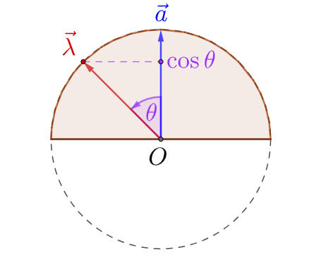
The image on the left demonstrates the measurement of spin by the parameter $\vec{\lambda}$, a unit vector, whose angle θ is also to the unit vector $\vec{a}$ in the direction from north to south of the magnet as the solitary partic-les pass through it. This represent-ation is logical as long as there is no other observer, when we can take the arc length of a circle, because a radian is just that, $\theta = \angle(\vec{a}, \vec{\lambda})$ is the arc length of the unit semi-circle spanned by these vectors. All projections of lambda that fall on the upper half have spin-up, while all proje-ctions outside the shaded semi-circle have spin-down. Lambda is the theoret-ical spin, it belongs to the superposition, and the projection is the value of the collapse and measurement.

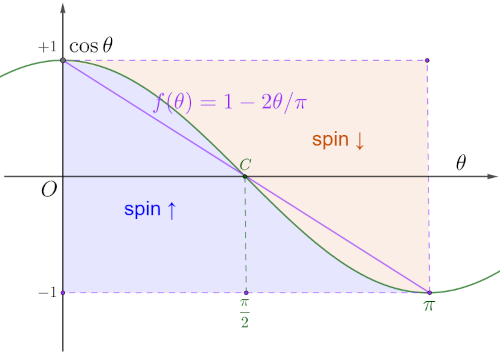
In the image on the right we see a graph of the same where below the purple straight line, f(θ) = 1 - 2θ/π, lies spin-up, and above it spin-do-wn, as we saw in a previous answer (Expected). Although correct for one particle, this insight does not coincide with the quantum graph, with the cosine line, in this image, but that does not matter much until other particles or other observers appear. How the discrepancy betw-een these two interpretations arises in the case of including others, I believe you can now see for yourself. This is what Bell also observed in his work.

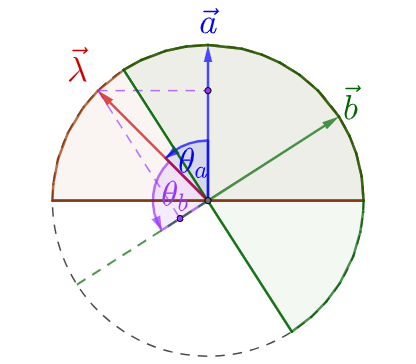
The questions just keep coming and I'll answer this one too. The new pi-cture of the left measurement is the spin of the Alice-Boban singlet, and perhaps the separation of current through two magnets. When the outcomes depend on the hidden parameter λ, and the angle between the two orientations is not zero, then unpleasant situations will ha-ppen. Superpositions fall both in the direction and the opposite. This spoils our quantum correlation ca-lculation, and leads to a contradic-tion (from the question we). Name-ly, it turns out that what we would measure and what we calculate are not the same, that is, that the very idea of ​​hidden parameters does not work.

Reset » srb

Question: What do you mean (Singlet, 3) that the last image, the Alice-Boban singlet spin measurement, is "perhaps also the separation of current through two magnets"?

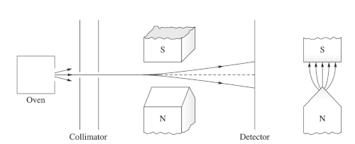
Answer: I suppose it's a bit confu-sing to think about "spin resetting," as the phenomenon I'm about to describe is sometimes called, and which comes from principled min-imalism, a concept unknown in physics today, but otherwise much broader. Let's go step by step.

1. In the picture on the right, a stream of atoms (silver) passes through a colli-mator, a device for creating a parallel beam, then through a magnet with a ve-rtically oriented north-south axis, which is then separated into two parts, an upper and a lower one. Spin-south particles go south, and spin-north go down. Spin is the essential form of angular momentum carried by elementary partic-les, and therefore also complex particles such as hadrons, atomic nuclei and atoms. Spin is conserved by a law similar to mass, energy or momentum, so we expect that by stopping the lower flow, that is, by taking only the upper one in the stream of atoms, there will be no more spin-down particles.

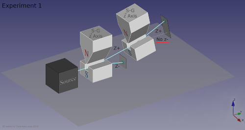
2. In the image on the left, the cur-rent of atoms is separated by the first magnet which is oriented south-north in the z-axis, so the upper current is passed through such a magnet once more and, indeed, there is no lower current. At this second exit, all the particles are with spin-up. Note that the same can be understood using Malus's rule, I = I₀ cos θ, which talks about the projections of the intensity of the cu-rrent. However, for now, it may seem as if the first magnet has "clean-ed" the flux of spin-down and therefore "naturally" only spin-up remains. The image has a link to Wikipedia.

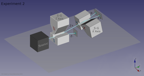
3. In the next picture on the right are the two previous magnets thr-ough which a current of particles flows, except that the second one (south-north) is tilted 90° relative to the first one. The second one takes only the spin-up particles of the first one but separates them again, right and left, we say into spin-up and spin-down relative to the x-axis. This completely destroys the old explanation that the first magnet "cleaned" the flux of spin-down particles and "left" only the spin-up particles.

What could be happening is a "resetting" of the spin orientation, with the gro-up of particles still having the same collective spin. We invest energy to start the wheel (Whirligig, 2), and it can continue to go round on its own until some other energy (force) stops it. Spin is the energy contained in these particles, which then have no "spin" (rotation) like a wheel or a top. This energy is inte-rnal to the particles themselves and does not include the directions of their polarization. The polarization of the particles themselves seems to tend tow-ards "disorder".

According to principled minimalism, or spontaneity towards greater probabi-lity and less information, or inaction, the development of thermal systems to-wards increasing entropy should be the path towards less information! What would be "disorder" to us, in the case of a broken glass, is actually a reduction in the total options (uncertainty) with which its pieces communicate. In the case of the aforementioned polarization of particles that "seem to tend towa-rds disorder", let us see returns to states of superposition, avoidance of dec-laration, minimalism.

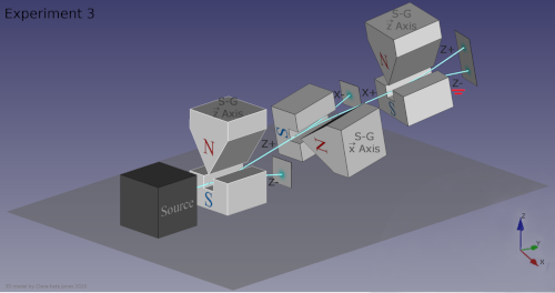
4. The new image on the left shows an even more complex and intere-sting experiment in three magnets. A beam of particles passes through the first, again vertical magnet, fr-om which the spin-up goes to the second horizontal one, while the spin-down is blocked. The one wh-ich passes encounters the vertical magnet and splits into two direct-ions, spin-up and spin-down. This would not be expected if there were trans-itivity in the correlation of these separations.

The correlation is not transitive, it is not transmitted as, say: the mixed set of even and odd numbers B has elements of the set of even numbers A, but has elements in common with the set of odd numbers C, while the sets of even A and odd C have no elements in common, when A ∩ B ≠ ∅ and B ∩ C ≠ ∅ it does not have to be A ∩ C ≠ ∅. Similar in this (Singlet, 3) is the Alice-Boban spin measurement with the separation of current (of silver atoms) through two magnets.

Due to the alleged resetting of the spin orientation, but not the change in the amount of spin, there is no transfer of orientations through the three magnets, no transitivity of correlation. The cause of the "resetting" of orientation, howe-ver, comes with the principle of minimalism, the spontaneous avoidance of emission and absorption of information, which is a consequence of the repu-lsive "force of uncertainty". Nature spontaneously tends to states of smaller choices, where it can, and that means inaction, because information transfers have actions as well as vice versa, and collapse is a strain on the superposition itself.

Linear » srb

Question: Can you explain to me more about the difference between parametr-ic (1 - 2θ/π) and quantum (cos θ) expectations, mean values?

Answer: I've included parts of that conversation (Oct. 2025) in the Fe-bruary blog replies (Expected). It was written in December 2025 for something else, but it can also serve as an introduction here, to the foll-owing.

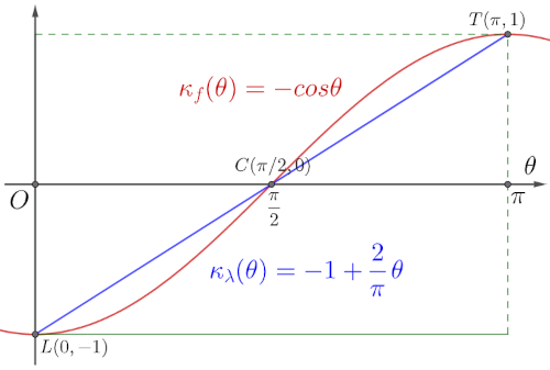
The image on the right is even better for such a topic. It follows the exposition of Bell's Theorem (1964), or rather the multitude of its explanations certainly better than my expositions (I believe, my style is not popular). The cosine curve κ_f(θ) = -cos θ ∈ (-1, 1) or "quantum" correlation, which I recently explained (Intensity, 5), intersects with the straight line of parametric correlation κ_λ(θ) = -1 + 2θ/π otherwise radians, the measure of the angle along the length of the unit circle. The two intersect at three points (L, C, T), which was also the subject of my recent blog (Singlet, 3).

1. The process of $\vec{\sigma}$ spin measurement is given by the Pauli matrices (Intensity, 3 and 4) and has eigenvalues ​​of ±1, which means that the measurements will give at most two values, spin-up and spin-down, with respect to $\vec{a}$, any unit ve-ctor of a given orientation of the Stern-Gerlach magnets. We use the notation from Bell's paper, and also consider a pair of fermions (half-integer spin) in a singlet spin state that are free to move in opposite directions. When in the first state $\vec{\sigma}_1\cdot\vec{a} = +1$ is measured, then in the second state $\vec{\sigma}_2\cdot\vec{a} = -1$ and vice versa. The hypothesis is introduced that there is a lambda parameter (whether it is a single variable or a set, or a set of functions, discrete or continuous), and further this λ is treated as a single continuous parameter.

The result A of the measurement $\vec{\sigma}_1\cdot\vec{a}$ is thus determined by $\vec{a}$ and λ, and the result B of the measurement $\vec{\sigma}_2\cdot\vec{b}$ at the same time is determined by $\vec{b}$ and the same λ, when:

$$ A(\vec{a},\lambda) = \pm 1, \quad B(\vec{b},\lambda) = \pm 1. $$

In this case, the result B of the second particle does not depend on the magnet $\vec{a}$, nor does the result A of the first particle depend on the setting of the magn-et $\vec{b}$. Let the probability density of the product of the aforementioned findings be ρ(λ), so the product correlation is:

$$ \kappa(\vec{a},\vec{b}) = \int A(\vec{a},\lambda)B(\vec{b},\lambda)\rho(\lambda)\,d\lambda, \quad -1 \le \kappa \le 1. $$

It should be equal to the quantum mechanical expectation:

$$ \langle \vec{\sigma}_1\cdot\vec{a}, \ \vec{\sigma}_2\cdot\vec{b}\rangle = - \vec{a}\cdot\vec{b} \in [-1,1], $$

and Bell proves that this is not possible. The hidden variables λ can be separ-ated into two sets, but given the breadth of the settings, this is also included here.

2. For example, if $\vec{b} = \vec{a}$, which corresponds to an angle θ = 0 between the po-larizations, and since the singlet state spin measurements opposites, A = -B, it will be:

$$ \kappa(\vec{a},\vec{a}) = \int(\pm 1)(\mp 1)\rho(\lambda)\,d\lambda = -\int\rho(\lambda)\,d\lambda = - 1, $$

and further (Singlet), we find three common values, the points L, C and T of the given image, and two correlations. Due to the assumed pair of singlet fer-mions moving freely in opposite directions, the coordinates of these points are L(0), C(π/2) and T(π). Also, the correlations are increasing functions of the angle θ ∈ [0, π] between the (unit vectors) polarizations. The well-known, quantum correlation (Intensity, 5), is thus reduced to the angle:

$$ \kappa_f(\theta) = - \vec{a}\cdot\vec{b} = - \cos\theta. $$

If we had only one particle (fermion) in a pure spin state with a given polari-zation, the unit vector $\vec{p}$, and we took only its spin-up through the magnet, then it is polarized spin-up. A unit vector $\vec{\lambda}$ that would have a uniform proba-bility distribution in the upper hemisphere would give $\vec{\lambda}\cdot\vec{p} \gt 0$. In this way, the hidden parameter follows the orientation of $\vec{p}$, only on one half of the sphere and not on the other. When compared to $\vec{a}$, one of the two states of the Stern-Gerlach experiment, it will give:

$$ \langle \vec{\sigma}\cdot\vec{a}\rangle = \vec{p}\cdot\vec{a} = \cos\theta. $$

So, we can also talk about some unit vector $\vec{a}'$ of the direction of a given polar-ization such that the measurement gives us the values ​​$\text{sign}(\vec{\lambda}\cdot\vec{a}')$, which are +1 for spin-up and -1 for spin-down, i.e. plus when lambda is in the hemisphe-re with polarization and minus when it is not. Between the upper and lower hemispheres (at the equator) the probability of lambda and this product are zero. According to this, now the expectation is $\langle \vec{\sigma}\cdot\vec{a}\rangle = 1 - 2\theta'/\pi$, where the angle $\theta' = \angle(\vec{a}',\vec{p})$, primarily because this probability distribution is uniform.

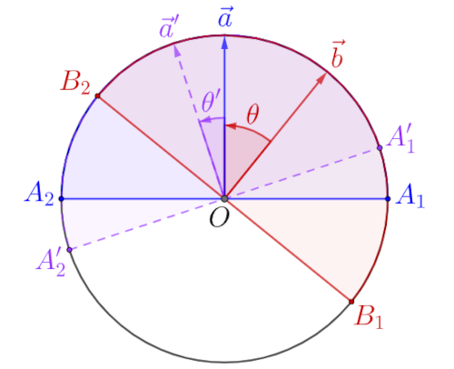
3. In the image on the left we see what happens when the lambda parameter tries to track polariza-tions. For an angle θ', the hemis-phere $\vec{a}'$ is tilted relative to the hemisphere $\vec{a}$, while this tilt is θ relative to another vector $\vec{b}$. Each of these corresponds to a straight line of correlation:

$$ \kappa_\lambda(\theta) = -1 + 2\theta/\pi, $$

but the beginnings of the angle me-asurements (θ = 0) are not equal, they do not start from the same points (A'₁, A₁ and B₁), nor do they have the same endings (A'₂, A₂ and B₂), so those straight lines do not coincide either.

As for Bell's theorem, it is enough to notice the discrepancy of one, any of the-se rectilinear graphs, with the cosine. In the upper right image, the red cosine is below the blue line for angles θ ∈ (0, π/2). This means a more negative qua-ntum correlation, κ_f < κ_λ, than expected by the hidden parameter. For angles θ ∈ (π/2, π) we have the reverse, but also a discrepancy κ_f > κ_λ. However, the cosine is stationary at the endpoints L and T, having a minimum and a maxi-mum with tangents parallel to the abscissa. This is not the case for a straight line, and it is another, subtle discrepancy, but mathematically sufficient to undermine the idea of ​​"hidden parameters." Bell noted this in his proof too.

Parameter » srb

Question: We discussed equations (9) in Bell's paper and couldn't agree on $B(a,b) = -\text{sign }\vec{b}\cdot\vec{\lambda}$. Can you explain that?

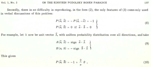
Answer: That's a slip of the pen. That mistake by Bell was also missed in the reviews. It should read (9):

$$ \begin{cases} A(\vec{a},\vec{\lambda}) = \text{sign }\vec{a}\cdot\vec{\lambda} \\ B(\vec{b},\vec{\lambda}) = -\text{sign }\vec{b}\cdot\vec{\lambda} \end{cases} $$

Open the image link on the right. There is a hypothesis, which Bell disputes, that there is a lambda parameter that determines the spin-up at location A so that the spin-down is measured at location B simultaneously. The observers at these locations in later literature are usually called Alice and Boban, and they are imagined to be so far apart that the speed of light cannot reach that simu-ltaneity, so Bell disputes the possibility that there is some other "hidden para-meter" (Einstein's proposal) of lambda that would allow the synchronization of measurements at these locations.

The positions A and B communicate only with this lambda, then a vector be-cause of the direction, which in the way of presentation can equally be a ma-trix or a tensor and the like. The assumption is that the measurement of pairs of quantum coupled fermions (half-integer spin) of total zero spin is observed, which move in opposite directions and hence opposite signs. Their only values ​​±1, are a special story about the intrinsic values ​​of spin measurement (Intens-ity). If this possibility of synchronization is also removed, using some hidden parameter, then quantum entanglement becomes a very strange phenomenon; at the same time Boban knows what Alice is doing even though they are very far away.

Namely, before the measurement, the direction of the spin is not a stated qu-antity, like the possible outcomes before rolling a dice. The spin is then a supe-rposition of multiple states that will collapse into just one of its possibilities. We measure that outcome. All of its information is exactly equal to the amou-nt of uncertainty that preceded it. In other words, the outcome of that singlet after the measurement for Alice leaves none of the previous uncertainty for Boban, which then means that Boban is left with only certainty. If the measu-rement for Alice gave spin-up, then for Boban it showed spin-down, and vice versa. Before the measurement, there was no way to predict the outcome in either of the two places, and suddenly, after measuring one, the results of both are known. That is the “magic” of quantum mechanics that confuses today’s science.

Unequal » srb

Question: Please also explain inequality (15) in Bell's paper to me, if you can, I can't seem to figure it out?

Answer: With that inequality:

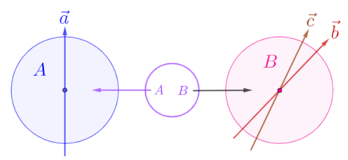
$$ 1 + \kappa(\vec{b},\vec{c}) \ge |\kappa(\vec{a},\vec{b}) - \kappa(\vec{a},\vec{c})| $$

Bell establishes a proof (Linear, 3) that the cosine shape, κ_f(θ) — of the quantum prediction, is stationary at both the endpoints L and T, that is, it has extrema and tangents par-allel to the abscissa, while the straight line of prediction with the hidden para-meter λ does not. Because of this difference, the idea of ​​hidden parameters is also bad for quantum mechanics. To explain this, as in this picture on the left, imagine that at B (Boban), in addition to $\vec{b}$ there is an alternative slightly incl-ined magnetic axis $\vec{c}$. That is the third (unit) vector of the given inequality of correlation (15).

1. Passing through the magnet, beam of the particles (silver atom) splits into two streams, we say spin-up and spin-down with respect to the (vertical) pole line of the magnet. Exactly as predicted by the Pauli matrices as operators (In-tensity, 3) of such a process. With the assumed parameter lambda measurem-ents of Alice and Boban can be $A(\vec{a},\vec{\lambda}) = \pm 1$ and $B(\vec{b},\vec{\lambda}) = \mp 1$. The norma-lized probability density distribution, ∫ ρ(λ) dλ = 1, gives their correlation (product) not less than -1 and not greater than +1:

$$ -1 \le \kappa_\lambda(\vec{a},\vec{b}) = \int A(\vec{a},\lambda)B(\vec{b},\lambda)\rho(\lambda)\,d\lambda \le +1. $$

This describes all possible spin directions within the superposition, before the collapse, before the measurement. However, $A(\vec{a},\lambda) = -B(\vec{a},\lambda)$, because Al-ice and Bob's outcomes are opposite due to the assumed zero total spin, so we have:

$$ \kappa_\lambda(\vec{a},\vec{b}) = -\int A(\vec{a},\lambda)A(\vec{b},\lambda)\rho(\lambda)\,d\lambda. $$

With the help of this remark, we obtain (15), here's how.

2. By substituting into the above correlation and subtracting, we find:

$$ \kappa_\lambda(\vec{a},\vec{b}) - \kappa_\lambda(\vec{a},\vec{c}) = -\int [A(\vec{a},\lambda)A(\vec{b},\lambda) - A(\vec{a},\lambda)A(\vec{c},\lambda)]\rho(\lambda)\,d\lambda = $$ $$ = \int A(\vec{a},\lambda)A(\vec{b},\lambda)[A(\vec{b},\lambda)A(\vec{c},\lambda) - 1]\rho(\lambda)\,d\lambda, $$

because $A(\vec{b},\lambda)A(\vec{b},\lambda) = (\pm 1)^2 = 1$. This is written in Bell's concise paper and it is now clear where it comes from: $A(\vec{b},\lambda)A(\vec{b},\lambda)A(\vec{c},\lambda) = A(\vec{c},\lambda)$, and A = ±1 also B = ±1. Because of the latter, however, we have and the following.

4. Finally, integrating the right-hand side of the previous inequality, is:

$$ |\kappa_\lambda(\vec{a},\vec{b}) - \kappa_\lambda(\vec{a},\vec{c})| \le 1 + \kappa_\lambda(\vec{b},\vec{c}). $$

The left side is the absolute value, because that side is smaller than the right side in both directions of subtraction. This is Bell's inequality (15) which wou-ld hold in quantum measurement (of Alice and Boban at the same time), I re-mind you, if it could be represented using hidden parameters. Bell then notes that this correlation is linear with the difference of angles, or with $|\vec{b} - \vec{c}|$, so $\kappa_\lambda(\vec{b},\vec{c})$ is not stationary at the minimum value (-1, when $\vec{b} = \vec{c}$) and conclud-es that this cannot be equal to the quantum mechanical value.

5.In cases where the angles between the orientations are larger, this inequality especially disagrees with the correlations derived from the assumed hidden parameter governing the spin outcomes for Alice and Boban. And the largest disagreement is for the angle 60°. Namely, then the quantum correlations are:

$$ \kappa(\vec{a},\vec{b}) = -\cos 60^\circ = - \frac12, $$ $$ \kappa(\vec{a},\vec{c}) = -\cos 120^\circ = \frac12, $$ $$ \kappa(\vec{b},\vec{c}) = -\cos 60^\circ = - \frac12, $$

so it is:

$$ |-\frac12 - (-\frac12)| \le 1 + (-\frac12), $$

i.e. 1 ≤ 1/2, which is clearly incorrect. So, assuming skewed parameters that would govern the outcomes of simultaneous spin measurements at distant locations of quantum entangled particles is a bad idea.

Criterion II » srb

Question: What is the use of an inequality, like Bell's (15) from 1964, when it is incorrect?

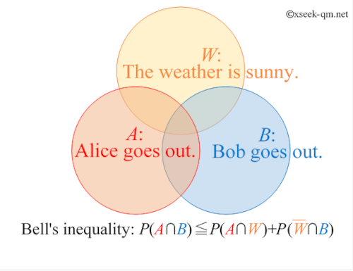
Answer: Bell's inequality and its later derivatives are convenient criteria for quantum entanglement, or more generally for testing the presence of a hidden parameter behind correlation in general. Simply put, Bell's inequality gives an upper bound on the probability that Alice and Bob will meet, as shown in the accompanying figure on the right, but as in that banal application, they hide a lot of useful physics and mathematics.

1. Everything revolves around the process $\hat{Q}$ as a linear operator and the que-stion of whether a pair of its vectors, states, or particles, singlet, is a quantum entanglement, and whose two matrix representations, Q' and Q'', are held by Alice and Boban.

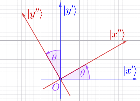
The image on the left shows a rot-ation by an angle θ with a pair of orthogonal vectors of some basis before and after the mapping:

$$ \begin{cases} |x''\rangle = \cos\theta |x'\rangle + \sin\theta |y'\rangle, \\ |y''\rangle = -\sin\theta |x'\rangle + \cos\theta |y'\rangle. \end{cases} $$

This is an example of a change that swap the set of eigenstates, the vec-tors $\vec{v}$ that are solutions to the cha-racteristic equation $\hat{Q}\vec{v} = \lambda \vec{v}$, as measured by Alice and Boban, but without changing their eigenvalues ​​λ. In this information theory, I stand by the unofficial interpretation (until further notice) that this quantum entanglement comes from the simultaneity of the observed particles or events themselves, which Alice and Boban do not see as simultaneous phenomena. In other words, a change in the vector space from the image is simultaneously reflected in both bases and we actually interpret this as quantum entanglement.

This seems very far from the criterion for "play" as a possibility in living but not inanimate beings, which it is not when we accept the uniqueness of the subjects of the universe (Riesz Lemma), also a specificity of this theory. This also includes the observation that Boban's measurement results take time to reach Alice, so these observations are abstractly simultaneous, i.e. quasi-simu-ltaneous. Like events now on Earth and imagined events "now" on a planet in some constellation in a galaxy billions of light years away.

2. A quantum state, vector |Ψ_s⟩, consists of two separable particles, respectiv-ely:

$$ |\psi_1\rangle = \alpha_1 |0'\rangle + \beta_1 |1'\rangle, \quad |\psi_2\rangle = \alpha_2 |0''\rangle + \beta_2 |1''\rangle, $$

where we use complex scalars and have the normalization, respectively:

$$ \alpha_1, \beta_1, \alpha_2, \beta_2 \in \mathbb{C}, \quad |\alpha_1|^2 + |\beta_1|^2 = |\alpha_2|^2 + |\beta_2|^2 = 1, $$

where |0⟩ and |1⟩ are the vectors of the standard basis, when it can be written as a tensor product:

$$ |\Psi_s\rangle = |\psi_1\rangle \otimes |\psi_2\rangle. $$

An non-separable quantum state would be:

$$ |\psi_n\rangle = \frac{1}{\sqrt{2}}(|0'\rangle\otimes |1''\rangle + |1'\rangle \otimes |0''\rangle). $$

It cannot be written in the previous way, using the tensor product of the given particles as separate individuals.

Inseparable particles are particles that Alice would measure in the state |0'⟩ and Boban would measure in the state |1''⟩ (simultaneously), or Alice would find the first particle in the state |1'⟩ and Boban in the state |0''⟩. Then they would be quantum entangled.

3. The Clauser-Horne-Shimony-Holt inequality (CHSH) is a key tool in quant-um physics, |S| ≤ 2, more details:

$$ |\kappa(\alpha,\beta) + \kappa(\alpha,\beta') + \kappa(\alpha', \beta) - \kappa(\alpha', \beta')| \le 2. $$

This inequality is derived from Bell's theorem and places limits on the correl-ations between measurements on separate particles. It is true when the parti-cles are governed by local hidden variables, only for local theories. However, statistical quantum mechanics predicts its violations up to 2√(2) for entangled particles, determining when nature is not locally realistic.

The source generates a pair of particles that Alice and Boban measure in their coordinate systems. Alice in the orthonormal bases $|0_\alpha\rangle$, $|1_\alpha\rangle$ and $|0_{\alpha'}\rangle$, $|1_{\alpha'}\rangle$, Bob in the orthonormal bases $|0_\beta\rangle$, $|1_\beta\rangle$ and $|0_{\beta'}\rangle$, $|1_{\beta'}\rangle$. We assign them:

$$ f_x = \begin{cases} 1, & |1_x\rangle \\ -1, & |0_x\rangle \end{cases} \quad \kappa(x,y) = \langle f_x\cdot f_y\rangle, \quad x \in \{\alpha, \alpha', \beta, \beta'\}. $$

These are four functions, two for Alice and two for Boban, which further defi-ne four correlations. If they satisfy the above inequality, then we are talking about a local action between Alice and Boban, otherwise about quantum ent-anglement.

4. For example, we observe the polarization of light through a vertical |1⟩ and a horizontal |0⟩ filter. Let the hidden parameter λ be the assumed angle of the photon. When a photon approaches the polarizer at some angle γ, it will be measured in the vertical state |1_γ⟩, or spin-up, if λ is closer to γ or γ+180° than to one of the angles γ±90°, otherwise it is in the horizontal |0_γ⟩ state, or spin-down. This is, therefore, the case where there is a hidden parameter.

This means that a measured photon with an assumed angle λ, the basis of the vertical |1_45°⟩ and horizontal |0_45°⟩ states, when it strikes at an angle from the first (from 0° to 90°) or third (from 180° to 270°) quadrant, we find the vertic-al state, i.e. +1. When it strikes at an angle from the second (90° — 180°) or fourth (270° — 360°) quadrant, we measure the horizontal state, i.e. -1.

Then, for Alice we have A(λ, α) = 1 when |λ - α| ≤ π/4 or |λ - α| > 3π/4, other-wise A(λ, α) = -1. For Bob B(λ, β) = 1 when |β - λ| ≤ π/4 or |β - λ| > 3π/4, oth-erwise -1. Then we calculate the integrals κ(α, β) = ∫ A(λ, α)B(λ, β)ρ(λ) dλ over values ​​of the angle λ. For the above (CHSH) inequality we calculate:

$$ S = \kappa(\alpha, \beta) + \kappa(\alpha, \beta') + \kappa(\alpha', \beta) - \kappa(\alpha', \beta'), $$ $$ S = \int A(\lambda, \alpha)B(\lambda, \beta)\rho(\lambda)\,d\lambda + \int A(\lambda, \alpha)B(\lambda, \beta')\rho(\lambda)\,d\lambda + $$ $$ + \int A(\lambda, \alpha')B(\lambda, \beta)\rho(\lambda)\,d\lambda - \int A(\lambda, \alpha')B(\lambda, \beta')\rho(\lambda)\,d\lambda, $$ $$ S = \int A(\lambda, \alpha)[B(\lambda,\beta) + B(\lambda,\beta')]\rho(\lambda)\,d\lambda + $$ $$ + \int A(\lambda, \alpha')[B(\lambda,\beta) - B(\lambda,\beta')]\rho(\lambda)\,d\lambda, $$

Since the values ​​of A, B are ∈ {+1, -1), these integral values ​​are either ±2 or 0. More precisely, if the value ±2 is inside the first of these integrals, then it is 0 in the second, and vice versa, if it is 0 in the first, then it is ±2 in the second. The value of the sum integral is therefore between -2 and +2, more precisely -2 ≤ S ≤ 2, i.e.

$$ |S| \le 2. $$

This is true in general when there are hidden variables.

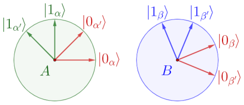
5. Another example is the quantum correlation whose data is given in the figure on the right. In red wou-ld be the measurements of Alice and Boban, again with the photon going to the polarizer with an angle γ. Again |1_γ⟩ and |0_γ⟩ are the verti-cal and horizontal polarizations. In quantum entanglement there is no hidden parameter λ. The correlation of the angles is the sum of the probabilities:

$$ \kappa(\alpha, \beta) = \Pr|1_\alpha 1_\beta\rangle - \Pr|1_\alpha 0_\beta\rangle - \Pr|0_\alpha 1_\beta\rangle + \Pr|0_\alpha 0_\beta\rangle. $$

We calculate probabilities by scalar multiplication, for example:

$$ \Pr|1_\alpha 1_\beta\rangle = |\langle \Psi | 1_\alpha 1_\beta\rangle|^2 = \frac12\cos^2(\alpha - \beta). $$

Thus, for the same pair of angles, we find:

$$ \Pr|1_\alpha 1_\beta\rangle = \Pr|0_\alpha 0_\beta\rangle = \frac12\cos^2(\alpha - \beta), $$ $$ \Pr|1_\alpha 0_\beta\rangle = \Pr|1_\alpha 0_\beta\rangle = \frac12\sin^2(\alpha - \beta). $$

For a given pair of angles, the above correlation is:

$$ \kappa(\alpha, \beta) = \frac12\cos^2(\alpha - \beta) - \frac12\sin^2(\alpha - \beta) - \frac12\sin^2(\alpha - \beta) + \frac12\cos^2(\alpha - \beta), $$ $$ \kappa(\alpha, \beta) = \cos^2(\alpha - \beta) - \sin^2(\alpha - \beta) = \cos[2(\alpha - \beta)]. $$

For example, let α = 0° and α' = 45°, so β = 22.5° and β' = -22.5°. Let's apply this correlation four times:

$$ S = \kappa(\alpha, \beta) + \kappa(\alpha, \beta') + \kappa(\alpha', \beta) - \kappa(\alpha', \beta') = $$ $$ = \cos 45^\circ + \cos 45^\circ + \cos 45^\circ - \cos 135^\circ, $$ $$ S = 2\sqrt{2}. $$

This value is greater than 2, the largest allowed by the (CHSH) inequality for correlations with a hidden parameter. Otherwise, it is S = 2√(2), the largest that can be obtained in quantum statistics where it can be less than 2. Howe-ver, for results greater than 2, we know for sure that Alice and Boban's obse-rvations are not driven by a hidden parameter, that there is one of quantum entanglement.

CHSH-Bell » srb

Question: What use do I have of Bell's inequality and how do you know that this CHSH is correct?

Answer: The topic of the discussion is that of the previous question Cri-terion II, but I am in the unusual situation of defending the imposs-ible thesis to the layman that there is nothing more useful than truth, for now only scientific or mathema-tical ones. I will prove this inequa-lity CHSH-Bell (1975), I hope, in a sufficiently general way that it will be applied at some point somewhe-re in ways that are currently, and perhaps even then, difficult for many to understand in everyday life.

1. So far, we have recognized quantum entanglement in the EPR paradox (1935), in Bell's theorem, using it specifically for the polarization of light, or in the Stern–Gerlach experiment guiding a beam through two polarizers or two magnets, but most often these are simultaneous measurements of the singlets of Alice and Boban. But the more recent Bell inequality (1975) allows for even looser assumptions in terms of proofs of the existence of hidden parameters, then the same cause for some seemingly unrelated measurements of Alice and Boban at distant locations at the same time. For example, Alice drives a car at speed α ∈ [-a, a] towards or away from Belgrade, while Boban drives another car at speeds β ∈ [-b, b] in the vicinity of Vladivostok, and we then wonder if there is some common cause, like hidden lambda parameters, their driving speeds.

2. So, we have Alice and Boban with values ​​α ∈ [-a, a] and β ∈ [-b, b] and in general from the set S_a and S_b respectively. The results of their measurements are two random variables x ∈ [-a, a] and y ∈ [-b, b], respectively. We need the joint probabilities, Pr(X, Y), of the sets of random events x ∈ X and y ∈ Y that two or more such events occur simultaneously. In mathematics, we usually denote them by Pr(X ∩ Y), the intersection of their occurrences, but this also means the probability of a 2-term sequence Pr(X, Y) implying the completen-ess (X, Y) as a unique "vector" of components of sets of random events. And here we also use the notations x ∈ S_a and y ∈ S_b to emphasize the entrants of Alice and Boban, some imaginary participants in physics experiments.

3. Conditional probability Pr(A|B) is the probability of event A occurring given that B has occurred. It reduces the possible outcomes (sample space A) to only those where the event in B has occurred. It is written as Pr(A|B), so:

$$ \Pr(A|B) = \frac{\Pr(A\cap B)}{\Pr(B)}. $$

This implies Pr(A ∩ B) = Pr(B) Pr(A|B), so Pr(B) Pr(A|B) = Pr(A) Pr(B|A), for any elements of the given sets of random events A and B. If we have Pr(A|B) = Pr(A), then we know that the events from A and B are independent. It is simil-ar in the case of joint events. In the above case Pr(X Y|λ) denotes the conditio-nal probability of realizing the outcome (x, y) ∈ (X, Y), under the condition of the presence of some random parameter λ ∈ Λ with probability q(λ) = Pr(λ). Sometimes we write probabilities with double-struck capital letter ℙ to distin-guish these functions from others, or simply P when there is no danger of confusion.

4. By viewing the conditional probability of joint events as a single vector-like sequence, it is easier to understand the following factorization:

ℙ_α,β(X, Y|λ) = ℙ_α(X|λ) ℙ_β(Y|λ),

which does not mean independence of conditional probabilities. However, fa-ctoring ℙ(X, Y) = ℙ(X) ℙ(Y) has meaning independence of the sets of random events X and Y. We apply this to two measurements, namely Alice with the number α some of the random variables x from the set X or S_a = [-a, a] and Boban with the number β from the random variables sets Y or S_b = [-b, b]. These probabilities depend on the parameters α and β which we will indicate by subscripting them. In particular, there is the presence of an (unknown) pa-rameter λ ∈ Λ which takes values ​​from some set Λ with probabilities q(λ). The locality follows from the written factorization of conditional probabilities. And I repeat all this too much because of the remarks of others that they find the proof extremely difficult to understand.

5. We can also write the required (CHSH-Bell) inequality in the form:

|Κ(α, β) + Κ(α, β')| + |Κ(α', β) - Κ(α', β')| ≤ 2ab,

where the correlation is defined by the expectation, Κ(α, β) = 𝔼_α,β(X, Y), which is valid for all α, α' ∈ S_a and all β, β' ∈ S_b. Then:

$$ K(\alpha, \beta) = \int XY\,d\mathbb{P}_{\alpha,\beta}(X,Y) = $$ $$ = \int dq(\lambda)\int XY\,d\mathbb{P}{\alpha,\beta}(X,Y|\lambda) $$ $$ = \int dq(\lambda)\, \int X\,d\mathbb{P}_\alpha(X|\lambda)\,\int Y\,d\mathbb{P}_\beta(Y|\lambda), $$ $$ K(\alpha, \beta) = \int dq(\lambda)\, \mathbb{E}_\alpha(X|\lambda)\,\mathbb{E}_\beta(Y|\lambda), $$

and this applied repeatedly gives the equalities:

$$ K(\alpha, \beta) + K(\alpha, \beta') = \int dq(\lambda)\,\mathbb{E}_\alpha(X|\lambda)[\mathbb{E}_\beta(Y|\lambda) + \mathbb{E}_{\beta'}(Y|\lambda)], $$ $$ K(\alpha', \beta) - K(\alpha', \beta') = \int dq(\lambda)\,\mathbb{E}_{\alpha'}(X|\lambda)[\mathbb{E}_\beta(Y|\lambda) - \mathbb{E}_{\beta'}(Y|\lambda)]. $$

By taking the absolute values ​​and adding them together, we find:

$$ |K(\alpha, \beta) + K(\alpha, \beta')| + |K(\alpha', \beta) - K(\alpha', \beta')| \le $$ $$ \le \int dq(\lambda)\,[|\mathbb{E}_\alpha(X|\lambda)| |\mathbb{E}_\beta(Y|\lambda) + \mathbb{E}_{\beta'}(Y|\lambda)| + $$ $$ + \int dq(\lambda)\,|\mathbb{E}_{\alpha'}(X|\lambda)| |\mathbb{E}_\beta(Y|\lambda) - \mathbb{E}_{\beta'}(Y|\lambda)|] $$ $$ \le \int dq(\lambda)\,2ab = 2ab. $$

This proves the required (CHSH-Bell) inequality.

6. A few explanations that may be unnecessary for experts will clarify the con-clusion of the proof for many. First of all, |x| ≤ a and |y| ≤ b are restrictions of random variables on the intervals S_a = [-a, a] and S_b = [-b, b] from which we take them. Therefore, the same restrictions also apply to the expectations (me-an values) of such variables, |𝔼_α(X|λ)| ≤ a and |𝔼_β(Y|λ)| ≤ b, and in the integ-rals these were factors in front of the absolute values ​​of the difference and the sum of the expectations. For the given sum of the difference and the sum, the generally known inequality holds:

|ξ + η| + |ξ - η| ≤ 2c,     ξ, η ∈ [-c, c],

which only needs to be applied twice under the integrals.

7. When the intervals are normalized, S_a divided by a and S_b divided by b, the random variables are restricted to the same interval x, y ∈ [-1, 1], and the resu-lt is that the correlation Κ(α, β) = 𝔼_α,β(X, Y) reduces to the prior κ(α, β). Then the above (CHSH-Bell) inequality will also become:

κ(α, β) + κ(α, β') + κ(α', β) - κ(α', β') ≤ 2

which we often refer to as CHSH Bell's inequality. It is understood that this left-hand side is also not greater than two if the previous (and abbreviated with ab) absolute value is not greater than two.

CHSH Game » srb

Question: Explain to me what the CHSH quantum entanglement game is?

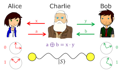
Answer: The letters CHSH come from the authors — John Clauser, Michael Horne, Abner Shimony, and Richard Holt — of the 1969 paper in which this “game” was discovered. They did not describe it as a game, but as an experiment. However, the description as a game is both natural and intuitive.

1. Alice and Boban are one team playing against referee Charlie, but they do not communicate with each other; A and B are like singlets. The referee sends a bit x to Alice and y to Boban, to get a response a from Alice and b from Boban depending on the strategy (x, y, a, b ∈ {0, 1}). The referee then compares the conjunction of his query, x ∧ y, the value 1 only when x = y = 1, with the answers in the exclusive disjunction, a ⊕ b, which is 1 only when a ≠ b. If it is established that x ∧ y = a ⊕ b, judge declares the team Alisa-Boban the winner in that exchange.

2. Alice's deterministic strategy is to answer a possible query x using one of the functions a: {0,1} → {0,1}. There are only four such:

1.     a(0) = 0     a(1) = 0,
2.     a(0) = 0     a(1) = 1,
3.     a(0) = 1     a(1) = 0,
4.     a(0) = 1     a(1) = 1.

If Boban also uses a deterministic strategy, combined with these four Alices, the Alice-Boban team has a total of 16 possible ways to deterministic answers. This is only a type of classical answer, which we distinguish in principle from quantum ones.

3. For example, Alisa-Boban decided that each of them would answer every question from the referee with 0. This is one of the deterministic strategies that can be described by the game table:

(x, y)	(a, b)	x ∧ y	a ⊕ b	point
(0, 0)	(0, 0)	0	0	⊤
(0, 1)	(0, 0)	0	0	⊤
(1, 0)	(0, 0)	0	0	⊤
(1, 1)	(0, 0)	1	0	⊥

After many repetitions of sending bits (x, y) from the judge to Alice and Boban that he (Charlie) chooses uniformly at random, the statistical number of positive (⊤) and negative (⊥) points tends to a ratio of 75-25 percent. Equal statistical winning effects are also produced by Alice and Boban's constant answers of 1 to all of the judge's queries. This 75 percent winning effect is actually the maximum for classical strategies.

4. The classic strategy and still deterministic would be in the negated answers. To query 0 both Alice and Boban answer with 1, and to query 1 they would answer with 0. The table of such a game is:

(x, y)	(a, b)	x ∧ y	a ⊕ b	point
(0, 0)	(1, 1)	0	0	⊥
(0, 1)	(1, 0)	0	1	⊤
(1, 0)	(0, 1)	0	1	⊤
(1, 1)	(0, 0)	1	0	⊥

Repeating this game, with random, uniform questions from the judge, would result in a 50-50 win-lose (⊤—⊥) split for the team of Alice and Boban. The same score is achieved by giving consistent answers when each player answers 0 on 0 and 1 on 1. These two strategies are worse than the previous two, and the random answer strategy is no better.

5. Let's now see how the Alice-Bob pair can achieve statistical wins of up to 85% with a quantum strategy. To do this, first look at some of the attachments to remind yourself of quantum notation and operators (Hadamard). A qubit is a vector and state of a quantum system:

$$ |\psi_\theta\rangle = \cos\theta |0\rangle + \sin\theta |1\rangle, $$

where each real number is an angle in radians. For example:

$$ |\psi_0\rangle = |0\rangle = \binom{1}{0}, \quad |\psi_{\pi/2}\rangle = |1\rangle = \binom{0}{1}, \quad |\psi_{\pm\pi/4}\rangle = |\pm\rangle = \frac{|0\rangle \pm |1\rangle}{\sqrt{2}}. $$

In the third case, it goes either plus or minus in all three places at once. The two states multiplied scalarly will give:

$$ \langle\psi_\alpha | \psi_\beta\rangle = (\cos\alpha\langle 0| + \sin\alpha \langle 1|)(\cos\beta|0\rangle + \sin\beta |1\rangle) = $$ $$ = \cos\alpha\cos\beta \langle 0|0\rangle + \cos\alpha\sin\beta \langle 0|1\rangle + \sin\alpha\cos\beta \langle 1|0 \rangle + \sin\alpha\sin\beta \langle 1|1 \rangle, $$

so because ⟨0|0⟩ = 1, ⟨0|1⟩ = 0, ⟨1|0⟩ = 0 and ⟨1|1⟩ = 1 we get:

$$ \langle\psi_\alpha | \psi_\beta\rangle = \cos(\alpha - \beta). $$

So much for the introduction with separable states.

6. However, to get a better score, Alice and Boban would have to enter an in-separable, coupled 2-qubit state (Criterion II, 2), and in particular a state of equal superposition when the probabilities of Alice and Boban's measureme-nts are equal:

$$ |\phi^+\rangle = \frac{|00\rangle + |11\rangle}{\sqrt{2}}. $$

You can find a short description of the otherwise complex calculation in the image link, and a more detailed description in the more serious lectures (CHSH strategy). The point is to work with two orthonormal bases, Alice and Boban, which can lead them to a quantum strategy with the expectation of maximum victory:

$$ \cos^2\frac{\pi}{8} = \frac{2 + \sqrt{2}}{4} \approx 0.85355 $$

and this is much more than (3/4 = 0.75) the best classical strategy.

7. Alice measures the received x bit in orthonormal bases:

$$ x = 0: \quad |\alpha_0\rangle = \binom{\cos\alpha_0}{\sin\alpha_0}, \quad |\alpha'_0\rangle = \binom{-\sin\alpha_0}{\cos\alpha_0}, $$ $$ x = 1: \quad |\alpha_1\rangle = \binom{\cos\alpha_1}{\sin\alpha_1}, \quad |\alpha'_1\rangle = \binom{-\sin\alpha_1}{\cos\alpha_1}, $$

where the angles α₀ = 0 and α₁ = π/4 = 45° for the expected maximum score, then the first basis vectors are |0⟩ and |1⟩, and the second basis vectors are |+⟩ and |-⟩. Note that the second basis is rotated by the first by an angle π/4.

On the other side is Boban who measures his received bit y in bases:

$$ y = 0: \quad |\beta_0\rangle = \binom{\cos\beta_0}{\sin\beta_0}, \quad |\beta'_0\rangle = \binom{-\sin\beta_0}{\cos\beta_0}, $$ $$ y = 1: \quad |\beta_1\rangle = \binom{\cos\beta_1}{\sin\beta_1}, \quad |\beta'_1\rangle = \binom{-\sin\beta_1}{\cos\beta_1}, $$

where its angles are β₀ = π/8 and β₁ = -π/8. Similar to Alice, Boban's second base is rotated first by an angle of -π/4, and in both cases the primed angle is the non-primed angle increased by π/2, i.e. α'_j = α_j + 90° and β'_j = β + 90° for both j = 0, 1.

8. Scalar multiplication (5) now gives ⟨ψ_α, ψ_β|Φ⁺⟩ = cos(α - β)/√2, and using this, and taking the upper angles, we quickly find the probabilities of the Alice-Boban team for the individual bits sent:

x = 0, y = 0:   |⟨α₀, β₀|Φ⁺⟩|² + |⟨α'₀, β'₀|Φ⁺⟩|² = cos²(α₀ - β₀),
x = 0, y = 1:   |⟨α₀, β₁|Φ⁺⟩|² + |⟨α'₀, β'₁|Φ⁺⟩|² = cos²(α₀ - β₁),
x = 1, y = 0:   |⟨α₁, β₀|Φ⁺⟩|² + |⟨α'₁, β'₀|Φ⁺⟩|² = cos²(α₁ - β₀),
x = 1, y = 1:   |⟨α₁, β₁|Φ⁺⟩|² + |⟨α'₁, β'₁|Φ⁺⟩|² = cos²(α₁ - β₁).

However, not all combinations of such angles are winning, nor will they always result in the best winning statistics. One of the best ones is for the given angles α₀ = 0, α₁ = π/4, β₀ = π/8 and β₁ = -π/8, when the first three of these combinations (x, y) give probabilities cos²(π/8) ≈ 0.85, which would be the best score.

This is just a sketch of a much more complex and precise calculation, of which there are many in quantum mechanics. The success of its calculation in exper-imental confirmations, which in terms of the accuracy of predictions surpasses anything previously seen in physics, seems to confirm the famous saying that “there is no free lunch.” When we gain in detail, we lose in complexity.

Analogy » srb

Question: I find this quantum mechanics difficult, I admit, but there must be some intuitive, easier explanation, for example, for the violation of Bell's ine-quality in cases of quantum entanglement?

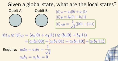
Answer: I get a lot of similar quest-ions that remind me of Richard Fe-ynman when he long ago claimed: when you think you understand qu-antum mechanics, then you don't understand it. Its problem, like that of excessive perfectionists with pro-bability theory, is that if you want to understand the causes that lead to the outcome of a coin toss, then you haven't understood the theory. The image link on the left reveals somethi-ng similar, and you will see exactly what it is from the explanation in my way.

1. Paraphrasing the video, using local quantum states (|ψ⟩_A = |0⟩, |ψ⟩_B = |+⟩) we can obtain the global state:

$$ |\psi\rangle_{AB} = |0\rangle\otimes|+\rangle = \frac{1}{\sqrt{2}}(|00\rangle + |01\rangle), $$

but it is not possible the other way around, we notice that by studying local phenomena we also learn about global phenomena, but that the reverse pro-cesses do not go so easily. Melting into the global, some local phenomena di-sappear without a trace (Localism) so that forms common to many remain (Global Convergence). That is why the experiment in physics can surprise us as much with its discoveries, especially of the ever-shrinking world but also of localisms in general, as the theoretical one manages to help us in connecting their differences. By analogy, these are differences to the uniqueness of the subjects of perception as opposed to abstract laws, like "everyone's", which are constantly repeated somewhere.

2. In this theory of physical reality, which implies that in a countably infinite sequence of moments with some infinite subsequence, one of at least two pos-sibilities is realized, there is a continuum (uncountably many) of possibilities. This, denoted by 𝔠, is an infinitely greater infinity than the discrete, denoted by ℵ₀, and is a type of "localism" that, through the outcomes and realizations of its possibilities, melts into the "globalism" of our reality. So how can we know all the options of that continuum from our real environment, when we are not even able to know all the physical phenomena that are before us as if on a platter.

3. There is also the answer to the question of the violation of Bell's inequality when quantum entanglement occurs. Just as the same circle within a smaller frame appears larger, or an even better example is the transition from a local quantum state to a global one (1), so the surviving quantities become compre-ssed and their importance grows, the correlations increase. Reductions of the local increase the visibility of the global, and then there is no going back, as in the operation of the principle of minimalism. Once you move into a more pro-bable state, into a less informative one, it is harder for you to go back to the less probable than to stay there among the then and smaller interactions.

4. Like a tight-fitting suit, Bell's inequality is bursting at the seams in the exc-ess of certainty, or what is the same, in the loss of uncertainty. So somehow I see the certain-uncertain as a kind of emptiness and fullness, where there is an almost arbitrary zero boundary and thinking of the Dirac vacuum. When there is less certainty of outcome and real information, then quantum entan-glement becomes visible. It is a state of mere present, too close to information, as well as beyond the reach of the speed of light, when quantum entanglement appears "out of nowhere".

Restriction II » srb

Question: Why is the Bloch sphere so successful for describing spin and corre-lations?

Answer: Because it's accurate, it's better at quantum interpretations of vectors, or it's simpler among other methods. Some of that is, I guess, and here's why that is.

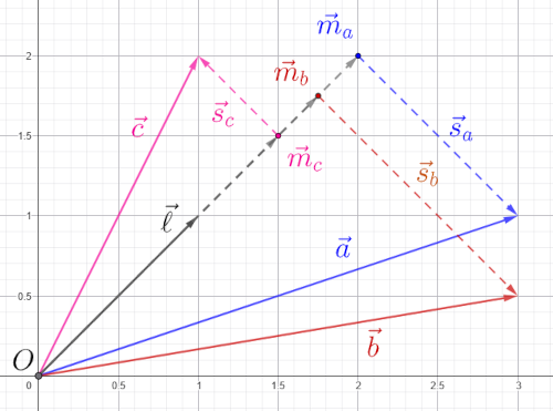
The image on the right is a 2-dim representation of the "stereometry of statistics" from my previous excerpt (Restriction), otherwise from the (unnoticed) book on information perception from back in 2016. The image shows vectors, sequences of random numbers:

$$ \vec{a} = (3, 1), \quad \vec{b} = (3, 0.5), \quad \vec{c} = (1, 2). $$

The mean values ​​(arithmetic averages) of their coordinates are, respectively, μ(a) = 2, μ(b) = 1.75 and μ(c) = 1.5. The bisector of that quadrant is directed by the vector $\vec{\ell}$ = (1, 1) which then determines the vectors $\vec{m} = \mu\vec{\ell}$, respectively:

$$ \vec{m}_{a} = (2, 2), \quad \vec{m}_{b} = (1.75, 1.75), \quad \vec{m}_{c} = (1.5, 1.5), $$

so the connectors are vectors:

$$ \vec{s}_a = \vec{a} - \vec{m}_a = (1,-1), $$ $$ \vec{s}_b = \vec{b} - \vec{m}_b = (1.25, -1.25), $$ $$ \vec{s}_c = \vec{c} - \vec{m}_c = (-0.5, 0.5). $$

They are perpendicular to $\vec{\ell}$.

1. Let's check the perpendicularity, that $\vec{s}_a$, $\vec{s}_b$, $\vec{s}_c$ ⊥ $\vec{\ell}$. Namely, vectors are perpendicular if and only if their scalar product is zero, so we calculate:

$$ \vec{s}_a\cdot \vec{\ell} = (1,1)\cdot (1,1) = 0, $$ $$ \vec{s}_b\cdot \vec{\ell} = (1.25, -1.25)\cdot (1,1) = 0, $$ $$ \vec{s}_c\cdot \vec{\ell} = (-0.5, 0.5)\cdot (1,1) = 0. $$

Therefore, the connectors of the given sequences of random numbers are indeed perpendicular to the bisector of the quadrant (of the rectangular Cartesian coordinate system).

2. According to the aforementioned excerpt, the correlation (Pearson's coefficient) is the scalar product of normalized connecting vectors:

$$ \kappa(\vec{a},\vec{b}) = 1, \quad \kappa(\vec{b},\vec{c}) = -1, \quad \kappa(\vec{c},\vec{a}) = -1. $$

Like measuring the spin of a particle with a magnet, there is complete correlation or complete anticorrelation. This is the success of the Bloch sphere, it uses only two real dimensions combined with Pauli matrices.

Note again, correlation is the cosine of the angle between the connectors, not between the random sequences themselves. The connectors of random varia-bles are always perpendicular to the quadrant bisector and, in the case of 2-dim nonzero sequences, the angle between them is either zero or stretched, so the cosine is 1 or -1. We can easily verify the given inequalities (Restriction, 3 and 4):

$$ \kappa_{bc}\kappa_{ca} - \sqrt{1 - \kappa^2_{bc}}\sqrt{1 - \kappa^2_{ca}} \le \kappa_{ab} \le \kappa_{bc}\kappa_{ca} + \sqrt{1 - \kappa^2_{bc}}\sqrt{1 - \kappa^2_{ca}}, $$ $$ 2\kappa_{bc}\kappa_{ca} - 1 \le \kappa_{ab}, $$

where the abbreviation is κ_ab instead of κ(a, b) and continues cyclically. These restrictions on the three correlations of three pairs of three n-tuples of rand-om variables should be distinguished from the three correlations κ(a, b), and κ(b, c) and κ(c, d) of four n-tuples of random variables for which there are no restrictions, because the correlation is not transitive.

3. The path from unit vectors of connections, to qubits, via the standard basis |0⟩ = (1, 0)^⊤ and |1⟩ = (0, 1)^⊤ to the pure states |ψ⟩ = α₀|0⟩ + α₁|0⟩, with com-plex numbers |α₀|² + |α₁|² = 1, is not far:

|Ψ⟩ = α₀|0⟩ + α₁|0⟩ =
= |α₀|e^iφ₀|0⟩ + α₁|e^iφ₁α₁|0⟩
e^iφ₀(|α||0⟩ + |α₁|e^{i(φ₀ - φ₁)}|1⟩,

and hence the usual "pure state" of a qubit:

|Ψ⟩ = |α||0⟩ + |α₁|e^iφ|1⟩.

Since cos²(θ/2) + sin²(θ/2) 1 for all θ ∈ [0, π], we write:

$$ |\Psi\rangle = \cos\frac{\theta}{2}\,\binom{1}{0} + \sin\frac{\theta}{2}\,e^{i\varphi}\binom{0}{1}, $$

and those unit vectors are actually points of the Bloch sphere.

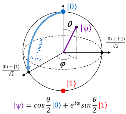
4. In the image on the left we see the Bloch sphere and vectors along the abscissa (x), ordinate (y), and applicate (z):

$$ |\pm\rangle = \frac{|0\rangle \pm |1\rangle}{\sqrt{2}}, $$ $$ |\pm i\rangle = \frac{|0\rangle \pm i|1\rangle}{\sqrt{2}}, $$ $$ |0\rangle = \binom{1}{0}, \quad |1\rangle = \binom{0}{1}. $$

Each point of such a unit sphere corresponds to a unique pair of angles θ and φ. For φ = 0, we obtain a great circle of the sphere in the abscissa-applicate plane (xz), and with φ = π/2 we have a great circle in the complex ordinate-applicate plane (yz). As we have seen, only one complex axis (y) extends the above 2-dimensional real system to the complex quantum mechanics.

We understand the addition of this imaginary y-axis as the freedoms that the particle in the superposition had before collapsing into just one of the two spin states (±). It is not possible to have them in reality. This is in accordance with the Copenhagen interpretation of quantum mechanics, advocated in the early 20th century by Bohr and Heisenberg, of quantum systems existing in a supe-rposition of all possible states until measurement, after which the wave func-tion "collapses" into a single state.

Strategy » srb

Question: Is it true that you use correlation to measure gaming strategies?

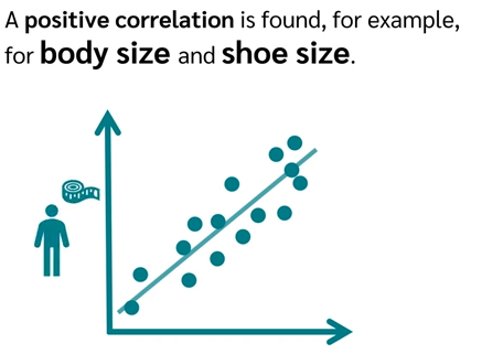
Answer: Yes, that's an unexpected discovery in the theory of Informa-tion of Perception, after I started using its basic idea in analyzing al-gorithms for some competitive ga-mes. See, for example, the link on image on the right to establish the more familiar concepts of correla-tion, and I'll continue with the less familiar ones.

1. In classical game theory, strategies are understood and refined models based on the von Neumann minimax theorem, in short, that subtracting the opponent's best moves is a good way to win. Similarly, corre-lation increases when we remove "bad" members from the arrays, designating them as those that are "good" for the opponent. It's not a simple question of how to value them, so let's leave that open. For now, let's stick to some kind of scale of numbers and, repeating a certain game, improve it step by step. For example, it can be values ​​from -1 to +1 real numbers, consistent with the recent answer (Expected, 4).

Note (CHSH Game) that correlation-determined strategies also apply to Nash equilibrium or even further examples of games than the von Neumanns. How-ever, the power of the "correlation method" for evaluating strategies is greate-st where classical game theory does not reach. Namely, the old so-called clos-ed and open games, such as poker and chess, or zero-level games (the first ga-ins as much as the second loses.), are generally too simple for situations when there are too many combinations or there is not enough time for the best mo-ve. And, additionally, when the opponent's moves come from all sides at once and similarly one has to respond to them, as in economics, politics or war.

2. From the sequences x = (ξ₁, ξ₂, ..., ξ_n) and y = (η₁, η₂, ..., η_n) we subtract the sequences μ_x ≠ 0 and μ_y ≠ 0, their mean values, to obtain the differences Δx_k = ξ_n - μ_x and Δy_k = η_n - μ_y, so the angle φ = ∠(x, y) is not equal to the angle γ = ∠(s_x, s_b). And the sequences s_x = (Δx_k) and s_y = (Δy_k) are the joins, that is, the vectors perpendicular to the quadrant bisector up to the given n-tuples (Restriction). The Pearson correlation, which is our topic, is the cosine of the angle between the joins (cos γ), not between the given sequences (cos φ), which makes the task a little more difficult. If you have nothing better, I rec-ommend starting with μ_x = μ_y = 0 and then using the trial-error-correction method, repeating the game, reach increasingly better average values.

3. The mean values ​​of μ of random events are expected, most likely in reality, and in this sense vital beings degenerate reality. Nature spontaneously tends to more probable states, which means fewer surprises, less communication, and less action. This includes the tendency to expect (μ) random events. Ho-wever, adding vitality to a natural process increases the odds, so we can move a glass on a table even when it could not move without us. In this way, the di-fferences Δx_k and Δy_k are measures of the action of vitality in the spontaneous natural flows of things, so that the cosine of the angle between the sequences s_x and s_y of these differences is a measure of the intensity of the skill of the game.

I describe the goals in forming the members of the arrays x and y. With them, we try to assess the opponents' vitality possibilities in the corresponding com-ponents of the game as accurately as possible. Building a strategy for a game becomes an interesting and not at all simple task. For a lone programmer it can be like building a skyscraper in front of a good mason with a trowel, mor-tar and bricks. When we leave it to machine learning, it gains momentum but loses some of its charm.

4. On the other hand, there are theoretical benefits to this method. Namely, given that the correlation is:

κ(s_x, s_y) = (s_x/∥s_x∥)⋅(s_y/∥s_y∥) = cos γ,
κ(s_x, s_y) = ξ₁η₁ + ξ₂η₂ + ... + ξ_nη_n,

which grows with the vitality of the players as the vitality of the game itself of the given players. And since the cosine is larger the smaller the angle γ, the vitality of the game is greater when the players are of similar abilities, when the vectors x and y are more parallel. Considering that the capacities of the players, the intensities ∥x∥ and ∥y∥ during the course of the game are not easily variable quantities and are measures of talent and previous preparations, then it is easier to deal with the redistribution of the intensity of the coefficients ξ_k and η_n in the sequence k = 1, 2, ..., n.

I mentioned this methodology (Win Lose), which is new to the well-known ga-me theory, but without the intention of popularizing it, and so its story waits in the shadows. In short, if you want to learn something from this, the so-call-ed reciprocity method is close to a good strategy, and based on the strength of success, it is also possible to describe the character of a person (Traits) again without a counterpart, for now, in the psycho or social sciences.

Transitivity » srb

Question: How will we transfer the intransitivity of correlation to strategy evaluations?

Answer: Naturally. Let's look at the magic square of numbers 3x3, in the picture on the left. Let's say that the columns are teams A, B and C, or more precisely the number of points they won in a competition. So team A played against B 2:7, 9:5 and 4:3, so with two wins and one loss they won the overall victory. Team B against C also won twice (7:6 and 5:1) and was defeated once (3:8), so they are the overall winne-rs. Again, team C is the winner of team A with two wins (6:2 and 8:4) and one loss (1:9).

So A > B > C > A, winning in team sports is not transitive, just as correlations are not transitive. We distinguish these from causality and deduction by reco-gnizing the contribution of vitality to games. Inanimate nature will not lie, will not play, nor can it defy the principle of least action from theoretical physics, and in this way it differs from vital living beings.

1. Transitivity is the mathematical operation of transfer. For example, a tree is a plant, a pine is a tree, so a pine is a plant. Similarly, transitive verbs like in "I cook lunch" where the subject (I) does something (cook) to someone or some-thing, unlike intransitive verbs like in the sentence "I grieve" where no one or nothing suffers the action, are not transferred. Formally, we consider transfers as inclusions (Latin inclusio), inclusions or encompassings as sets. In the con-text of sets A ⊆ B it means that set A is contained in B, so if B ⊆ C then A ⊆ C. This is transitivity.

2. One of the more commonly mentioned but also general examples of non-transitivity of correlation is with three independent normal (Gaussian) dist-ributions of random variables A, B and C by which we define three new ran-dom variables X = A + B, then Y = B + C and Z = C - A. The correlation betw-een the first two corr(X, Y) = 0.5 is positive, the correlation between the sec-ond and third corr(Y, Z) = 0.5 is also positive, but the third correlation with the first is negative corr(Z, X) = -0.5. This shows that strong pairwise correla-tions are not transmitted in a chain and will not ensure correlation between end elements.

You will find many concrete examples of correlation intransitivity, such as the following. A is a fruit salad made from papaya and banana, B is a fruit salad made from banana and strawberry, C is a dish made from strawberries and cream. When the price of bananas increases, the prices of salads A and B in-crease, so A and B are positively correlated. When the price of strawberries increases, the prices of B and C will increase, so B and C are positively corre-lated. However, A (papaya and banana) and C (strawberries and sour cream) have no ingredients in common, so their price correlations will likely be close to zero, their prices will be uncorrelated.

3. We distinguish three types of (un)connection of phenomena: randomness, correlation and causality. Complete unconnection is a uniform distribution, when all outcomes are equally likely. We see ultimate connection in theorems, as in the formula 2 + 3 = 5 with its certainty that two "somethings" and three of the same give five of them. The greatest information (Extremes) have equal probabilities on a given interval (a, b), then exponentially decreasing with a certain expectation μ, then normal (Gaussian bell) with a given dispersion σ. Due to the principle of Minimalism, nature will spontaneously emerge from such, and will slide from randomness to connection.

4. The central limit theorem applies the weak laws of large numbers to proba-bility theory and states that the sum of a large number of independent random variables X_k, where k ∈ {1, 2, ..., n}, with equal means μ and variances σ², ten-ds to a normal probability distribution. Thus, that:

$$ Y_n = \frac{X_1 + X_2 + ...+ X_n}{n} $$

almost certainly converges to expectation μ and variance σ² when n → ∞. This has the limiting form of the distribution:

$$ Z = \lim_{n\to \infty} \sqrt{n}\left(\frac{Y_n - \mu}{\sigma}\right), $$

and that is the normal (Gaussian) probability distribution. There are various versions of the same theorem, in some of which it is not necessary for the va-riables to have the same probability distribution, if no variable has a dominant influence on the final sum. I mention them here to note the laws of large num-bers with their powers of shaping uncertainty, long known.

5. We also define the uniform distribution 𝒰(a, b) with a probability density (Physical Information, p. 64):

$$ \rho_{\mathcal{U}}(x) = \begin{cases} \frac{1}{b-a}, & x \in [a, b] \\ 0, & x \notin [a, b] \end{cases} $$

where a < b. Its expectation and variance are then:

$$ \mu_{\mathcal{U}} = \frac{b + a}{2}, \quad \sigma^2_{\mathcal{U}} = \frac{(b - a)^2}{12}, $$

and information:

$$ S_{\mathcal{U}} = \ln(b-a). $$

Normal distribution 𝒩(μ, σ²) is defined by the density:

$$ \rho_{\mathcal{U}}(x) = \frac{1}{2\pi\sigma^2}e^{-\frac{(x - \mu)^2}{2\sigma^2}}. $$

Its expectation is μ, variance σ² and (Physical Information, p. 68) information:

$$ S_{\mathcal{N}} = \ln\sqrt{2\pi e\sigma^2}. $$

Substituting the previous variance into this one, we find:

$$ S_{\mathcal{N}} = \ln\sqrt{2\pi e\frac{(b-a)^2}{12}} = \ln(b-a) + \ln\sqrt{\frac{\pi e}{6}}, $$ $$ S_{\mathcal{N}} = S_{\mathcal{U}} + 0.176... $$

which means that the information of the normal distribution (S_𝒩) is about 0.176 greater than the information of a single uniform distribution (S_𝒰), but this is too little considering the long series of uniform distributions X₁, X₂, X₃, ... that participate in the formation of the normal distribution. This deficit, I believe, is due to the principle of minimalism.

Spearman » srb

Question: Pearson's correlation is linear, but Spearman's is not?

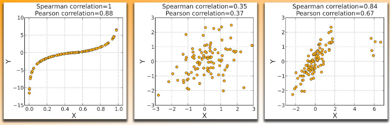
Answer: Yes, unlike Pearson's correlation, which looks for a linear relation-ship, Spearman's method is more flexible and can handle nonlinear correla-tions. In the image above, three comparison cases are shown. In the first gr-aph, the Spearman correlation coefficient is maximal (ς = 1), because they compare two variables (x_i, y_i) that are monotonically related (both increasi-ng), although their relationship is not linear. But the same pairs give a less than perfect Pearson correlation (κ = 0.88).

In the second (middle) graph, of data with an approximately elliptical distrib-ution, without prominent anomalies, Spearman's (ς = 0.35) and Pearson's (κ = 0.37) correlations give similar values. In the third (right) graph of the same figure, Spearman's correlation (ς = 0.84) is less sensitive than Pearson's (κ = 0.67) to strong outliers located in the tails of both samples. Spearman's ς then ignores the outliers and is limited to the values ​​of the remaining domains. The common notation for Pearson's correlation coefficient is r, Spearman's ρ, and the latter is generally similar to Kendall's is usually denoted τ. The latter two are rank-based coefficients; they are nonparametric correlations, and unlike Pearson's so-called parametric ones.

1. The formula for Spearman's correlation is:

$$ \rho = 1 - \frac{6\sum d^2_i}{n(n^2-1)} $$

where the random variables are ranked, their order of values ​​is formed, and then the differences d_i = x_i - y_i are taken for all i = 1, 2, ..., n of their rank, whi-ch are squared and summed. In detail, let's look at an example of calculating Spearman's correlation of the success of ten students in two tests, English and mathematics. They received the following scores, respectively:

English:           56     75     45     71     62     64     58     80     76     61
Mathematics:   66     70     40     60     65     56     59     77     67     63

We rank each one separately, in a top-list from best to worst:

English:           9     3     10     4     6     5     8     1     2     7
Mathematics:   4     2     10     7     5     9     8     1     3     6

Then we calculate the differences and squares of the differences:

d:       5     1     0     3     1     4     0     0     1     1
d²:   25     1     0     9     1     16     0     0     1     1

We add the squares of the differences and insert them into the above formula:

$$ \rho = 1 - \frac{6\sum d^2_i}{n(n^2-1)} = 1 - \frac{6\cdot 54}{10(10^2-1)} = 1 - \frac{324}{990} \approx 0.673 $$

This is a strong positive relationship between demonstrated success and the ranks individuals achieved on the mathematics and English language exams, i.e., those who were ranked higher in mathematics were also ranked higher in English, and vice versa.

2. In the image on the right is a link to another example with the same correlation explained in a little mo-re detail, this time with eight com-puter gamers whose reaction times were measured in comparison to their ages. The column below the clock is sorted, the age column is joined to it so that we can easily calculate the differences:

d₁ = 1 - 1 = 0
d₂ = 2 - 3 = -1
...
d₈ = 8 - 8 = 0

The sum of the squares of these differences is 8, and the number of participants n = 8, so we calculate Spearman's correlation:

$$ r_s = 1 - \frac{6\cdot\sum_{i=1}^8 d^2_i}{n(n^2-1)} = 1 - \frac{6\cdot 8}{8(8^2 - 1)} = 0.9047619... $$

This is a very strong correlation. Increasing age correlates strongly with lengthening of reaction time (reflex). This appendix additionally contains comparisons of Pearson, Spearman, and Kendall correlations, and also pro-vides an explanation of hypothesis testing. I would add that in the case of so-me equal values ​​​​using which we create a top list, we should take the average rank value and assign it to all of them.

3. An Indicator is a function 1_A(x) ∈ {1, 0} defined on a set A for which 1_A(x) = 1 when x ∈ A, but 1_A(x) = 0 if x ∉ A. It is often accompanied by a probability that x belongs to the set A which is p ∈ (0, 1), that is, x does not belong to the set A such that q = 1 - p. Among others, indicators are one of the topics of my book Physical Information (p. 71).

Let us now consider the repetition of the same random experiment until the first occurrence of a “favorable” event (probability p). The probability that a favorable outcome will occur in the first attempt is p, and that an unfavorable outcome will occur first and then favorable is qp. The probability that a favo-rable outcome will occur only in the third repetition is q²p. In general, the probability that a favorable outcome will occur for the first time only in the nth attempt is q^n-1p, because before that, an unfavorable outcome with prob-ability q = 1 - p has occurred n - 1 times. Given two probabilities p_x = 0.5 and p_y = 0.6, we calculate two such sequences:

n	px = 0.5		py = 0.6
1	0.500		0.600
2	0.250		0.240
3	0.125		0.096
4	0.062		0.038
5	0.031		0.015
6	0.016		0.006
7	0.008		0.002
8	0.004		0.001
9	0.002		0.000
10	0.001		0.000

These are infinite sequences that converge exponentially, so after just these 10 steps, the sum of the first has accumulated approximately z_x = 0.999023 and the sum of the second z_y = 0.999895.

I give them as an example of equally ranked Spearman correlation and there-fore exactly 1. They are maximally correlated according to Spearman's meth-od, but not in the Pearson way. Namely, the mean values ​​of the trials are μ_x = 1/p_x = 1/0.5 = 2 and μ_y = 1/p_y = 1/0.6 = 5/3, so the sequences s_x and s_y are different (Restriction) so the Pearson correlation κ is not exactly 1.

4. However, the deeper motive of this example is the search for the possibility of varying the local freedoms of the eventual participants of the information perception while the overall capacities of each of them do not change. Without these possibilities, the meaning of strategies disappears, at least not in the domain of changing the strength of an individual's game despite his (lack of) talent. The sorting and measurement criteria of different methods of correla-tion testify in favor of these possibilities, creative improvement or weakening of the game, but when we look closely, they are also just one form of local div-ergences (Localism) and global convergences.

Monotonic » srb

Question: Spearman's correlation is less sensitive to the causes of the relation?

Answer: It's an unusual thing to say, but it's true. Looking at mere rankings, comparing the tourna-ment participants' rankings, and the top lists of points won, we have no direct insight into the efforts made by the participants. Hence the differences in these measur-ements, Spearman and Pearson. And in the long run, effort and talent do their job, and yet it turns out that statistics (repetition of patterns) act through the laws of large numbers, that the past influences the future, as if such phenomena are crying out for reality.

1. Monotonicity is doubly desirable here. First, for the sake of ranking, order-ing the values ​​of the raw data, the random variables. And secondly, it comes from the need for consistency, the aforementioned formation of the "past" that would influence the "future". First of all, let's make sure that the form of Spe-arman's correlation and Pearson's, that one reduces to the other when from the raw data:

x = (ξ₁, ξ₂, ..., ξ_n),     y = (η₁, η₂, ..., η_n),

Let's move on to the rank of one and the other. When we sort each of these two arrays by size, their original comparative elements will be unpaired, their placements may change their order. Let the ordinal number of element ξ_k be ξ'_k, and let the ordinal number η_k be η'_k. Thus we find two arrays of ordinal numbers from the set {1, 2, ..., n}, unsorted:

x' = (ξ'₁, ξ'₂, ..., ξ'_n),     y' = (η'₁, η'₂, ..., η'_n),

If we were to sort the first one so that it is monotonically increasing (or decre-asing), the second one does not have to be so, and it is precisely their possible difference that affects the (non)correlation in Spearman's sense. There can be a lot of freedom to change the values ​​of individual members of the raw arrays, x or y, but so that their order x' or y' remains the same.

2. Let's check that the Pearson correlation of the ranged the given lists:

$$ \kappa(x', y') = \frac{\text{cov}(x',y')}{\sigma(x')\sigma(y')} $$

of raw arrays of values ​​x and y give Spearman's correlation:

$$ \varsigma(x,y) = 1 - \frac{6\sum_{k=1}^n d^2_k}{n(n^2-1)} $$

where the random variables are ranked in order of value, and then the diff-erences d_k = ξ'_k - η'_k are taken for all k = 1, 2, ..., n of their orders, which we square and then add.

3. To calculate the covariance, both are sequences from the set {1, 2, ..., n}, we look for the mean of these sequences. It is the nth part of the arithmetic mean A of the sequence, so let's calculate it first. Let's write it like this:

A = 1 + 2 + ... + (n-1) + n,
A = n + (n-1) + ... + 2 + 1

and add them. We get:

2A = [1 + n] + [2 + (n-1) + ... + [(n-1) + 2] + [n + 1],

A = n(n + 1)/2,     μ = A/n = (n + 1)/2.

The first (A) is the well-known formula for the sum of the first n natural num-bers, and the second (μ) is the desired mean value that we need for the covar-iance.

Equally ranked would be those with equal starting values, e.g. ξ_i = ξ_j, to which we assign the mean value, (ξ'_i + ξ'_j)/2. For example, when positions 6 and 7 have the same starting values, both receive a rank of 6.5. Then we should dis-tinguish the expectation E(x') = μ_x' from E(y') = μ_y', otherwise not.

4. To calculate the variance, we look for the mean of the sum of the squares of B of the same numbers. We have B in the differences of the cubes, from 1 to n, which we add up:

$$ \sum_{k=1}^n [k^3 - (k-1)^3] = \sum_{k=1}^n [k^3 - (k^3 - 3k^2 + 3k - 1)], $$ $$ n^3 = \sum_{k=1}^n (3k^2 - 3k + 1) = 3B - 3A + n, $$ $$ B = \frac13 n^3 + A - \frac13n = \frac{n(n+1)(2n+1)}{6}, $$ $$ \sum_{k=1}^n k^2 = \frac{n(n+1)(2n+1)}{6}, $$ $$ \sigma^2 = \frac{1}{n}B - \mu^2 = \frac{n^2 - 1}{12}. $$

When all ranked numbers ξ'_k, η'_k are ∈ {1, 2, ..., n}, then σ_x' = σ_y' and μ_x' = μ_y'.

5. Then, we calculate (2):

$$ \kappa(x',y') = \frac{E(x'y') - E(x')E(y')}{\sigma(x')\sigma(y')} = \frac{\frac{1}{n}\sum_{k=1}^n\xi'_k\eta'_k - \mu_{x'}\mu_{y'}}{\sigma_{x'}\sigma_{y'}}, ... $$

Let's note that the numerator states:

$$ \frac{1}{n}\sum_{k=1}^n\xi'_k\eta'_k - \mu_{x'}\mu_{y'} = \frac{1}{n}\sum_{k=1}^n \frac12[\xi'^2_k + \eta'^2_k - (\xi'_k - \eta'_k)^2] - \mu_{x'}\mu_{y'} = $$ $$ = \frac12\frac{1}{n}\sum_{k=1}^n \xi'^2_k + \frac12\frac{1}{n}\sum_{k=1}^n \eta'^2_k - \frac{1}{2n}\sum_{k=1}^n d^2_k - \mu^2 $$ $$ = \left(\frac{1}{n}\sum_{k=1}^n \xi'^2_k - \mu^2\right) - \frac{1}{2n}\sum_{k=1}^n d^2_k $$ $$ = \sigma^2_{x'} - \frac{1}{2n}\sum_{k=1}^n d^2_k $$ $$ = \sigma_{x'}\sigma_{y'} - \frac{1}{2n}\sum_{k=1}^n d^2_k. $$

Putting this back into the numerator and substituting (4), we get:

$$ \kappa(x',y') = \frac{\sigma_{x'}\sigma_{y'} - \frac{1}{2n}\sum_{k=1}^n d^2_k}{2n\cdot\frac{n^2-1}{12}} = 1 - \frac{6\sum_{k=1}^n d^2_k}{n(n^2-1)}, $$

and this Pearson's κ(x', y') is Spearman's ς(x, y), above.

6. What we perceive is never what “is” (there is no such thing), but rather dual images (Conjugated) and are never completely the same in different subjects, moreover, they are not the same even in the same participant in communica-tion at different times (Information Coupling, p. 124). On the other hand, the-re is no decisive discussion of “causes” based solely on correlation (Transitivi-ty, 3), so the question posed becomes out of place. However, I took the oppor-tunity to emphasize that the duality of perception and the uniqueness of subj-ects cooperate with correlations.

Kendall rank » srb

Question: I don't understand this Kendall rank correlation coefficient on Wikipedia. Can you explain to me?

Answer: See the explanation with the image on the right. It's better than any of my stories and I can probably just comment on it in case the video doesn't open, or your Serbian is better than English (to anyone online). Additionally, I'm saving this answer for later.

In this picture, for example, we have two people with ranked su-ccesses in six disciplines, or in six tests. We want to check the correlation of their skills, or knowledge. The disciplines are ordered according to the successes of the first participant, and the rankings of the second are next to each other. Where the first has the best success (rank 1), the second is only third (rank 3). When the person on the left is with rank 2, the right is with rank 1, when the left wins third place, the right is fourth, and so on down the table.

Then we look at the ranking of the right participant himself, from top to bott-om. In the first position (number 3) it is less than the three numbers below {4, 6, 5} and greater than the two {1, 2}, which means that it is three times Conc-ordant and two times Discordant with the ranking order. The next one (numb-er 1) is less than all four below, that is, it is 4 times Concordant and 0 times Discordant with the ascending table of the left participant. The third one in line (number 4) is twice Concordant and once Discordant. The next one (number 2) is both Concordant, and then comes the number (6) which is not in agreement with the only one (5) below it. Agreements are in the columns on the right "pluses" and there are C = 11 of them, and disagreements are "minus" and there are D = 4. The Kendall correlation coefficient is:

$$ \tau = \frac{C - D}{C + D} = \frac{11 - 4}{11 +4} = \frac{7}{15} = 0.47. $$

And that's it. Like the Pearson coefficient, this Kendall τ ∈ [-1, 1] has the same meaning. Total correlation will be τ = 1, the absence of any correlation will give τ = 0, and anticorrelation (one increases, the other decreases) is τ = -1. Quick description:

   0.1 ≤ τ ≤ 0.1   no correlation,
   0.1 ≤ τ ≤ 0.3   weak correlation,
   0.3 ≤ τ ≤ 0.5   medium correlation, 
   0.5 ≤ τ ≤ 0.7   strong correlation,
   0.7 ≤ τ ≤ 1.0   very strong correlation.

The Kendall tau coefficient is generally smaller than the Spearman coefficient (usually denoted by ρ) and is better for smaller arrays, say at least 40 elemen-ts. Certainly larger than the 6 in this example. In games, the application of Kendall's tau coefficient is a bit more convenient than the previous two. It is faster, uses less memory, and is easier to reduce to real-unreal, or true-false during ongoing evaluations and player management towards victory.

As a reminder, in applying this theory to complex games of winning, a coincid-ence of better position reading and “reciprocal” (timely, measured, and creati-ve) response with success is shown. More specifically, when a specific “amount of truth” can be measured (Packages III), it also coincides with strong action.

February 2026 (Original ≽)