January 2026 (Original ≽)

Lambert » srb

Question: Can you solve the problem t^t = 21 for me?

Answer: I don't deal with math in-structions, but this particular prob-lem is a handy example of the met-hod sometimes needed for functi-ons of the form x⋅ln(x) which are also sums in Shannon's informat-ion sum.

1. The natural logarithm of the ar-gument x is the function y = ln(x) inverse to the exponential y = e^x, so the two cancel out:

ln(e^x) = x,     e^ln(x) = x,

with base e = 2.71828... When we take the logarithm of the equation from that problem, first ln(t^t) = ln(21), then inversely t^t = e^ln(21), then we take the root t = e^ln(21)/t and back inversely ln(21)/t = ln(t). Multiplying by the denominator ln(21) = t⋅ln(t) and:

t⋅ln(t) = ln(21)

and we find what we otherwise know about logarithms of arbitrary base b, that log_b(xⁿ) = n⋅ln(x). We introduce the substitution t = e^x and get:

x⋅e^x = ln(21).

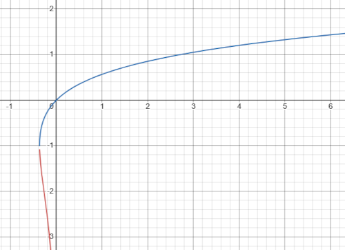
Next, we need the Lambert W function, whose graph is in the image above.

2. The Lambert W function is defined by the equality:

W(ze^z) = z,     z ∈ ℂ.

We apply it to both sides of the previous equality and return the substitution:

W(xe^x) = W(ln 21),
x = W(ln 21),
ln t = W(ln 21),
t = e^{W(ln 21)},
t ≈ 2,879.

Calculators, or sometimes tables, of Lambert's W function can be found along with logarithms or trigonometric functions. For example, the site Wolfram-Alpha has an option where you can type exp(LambertW(ln(21)) online to get the specified result. Check 2.879^2.879 = 20.996976... ≈ 21.

3. In the Python (3.11.0) programming language, enter:

import numpy as np
from scipy.special import lambertw
a = np.log(21)
b = lambertw(a)
c = np.exp(b)
print('exp(W(ln(21)) =', c)

You will receive:

exp(W(ln(21))) = (2.8790699928935655+0j)

That's also the result from the WolframAlpha calculator.

4. Example. Let's solve the equation 3^x - 4x = 5.

Solution: We prepare the given expression for the Lambert W function:

3^x = 4x + 5,     / ⋅3^-x
1 = (4x + 5)⋅3^-x,     / ⋅(-1)
-1 = -(4x + 5)⋅3^-x,     / :4
-1/4 = -(x + 5/4)⋅3^-x,     / ⋅3^-5/4
-3^-5/4/4 = -(x + 5/4)⋅3^{-(x + 5/4)},
-(3^-5/4ln 3)/4 = -(x + 5/4)(ln 3)⋅e^{-(x + 5/4)ln 3}.

Next, we apply Lambert's W function and calculate the unknown:

W[-(3^-5/4ln 3)/4] = W[-(x + 5/4)(ln 3)⋅e^{-(x + 5/4)(ln 3)}],
-0.06956 ≈ -(x + 5/4)ln 3,
-0,06956/1.09861 ≈ -(x + 5/4),
-0.0633 ≈ x + 5/4,
x ≈ -1.187.

Checking 3^x - 4x = 5.018 confirms the approximate solution x ≈ -0.862. ∎

Toaster » srb

Question: Explain to me this concept of a pseudo-universe and an intelligence that is necessarily deceitful and prone to corruption?

Answer: That was a story from al-most ten years ago, with some hy-pothetical beings, let's say, about extraterrestrial intelligences. But now there are increasingly powerful computers, so imagine them, that we might be talking about them, about some even more developed similar artificial intelligence.

1. We fantasized about it more than I wrote, but I found one story pres-erved, "Dualism Lies" (Information Stories, p. 106), yet it's not very detailed. Read it first (again if it is necessary)

Note that the emphasis here is on the possibility of deciphering lies, the chan-ce that by sending false messages someone will receive a hidden correct mes-sage. Not everyone will be engaged in deciphering, nor is every key for every lock; we are not given the opportunity to communicate with everyone. Follo-wing this trail, we come across an important discovery, that a lie is less infor-mative than the truth. Untruth is, for the most part, a diluted truth. Hence the appeal of lies. Nature prefers less action, less communication, less informati-on, that is, it will more often realize more likely random outcomes.

2.The second piece of the puzzle to answer the question I was asked is found in the (also new) considerations of “Islands” as places where truths reside. Th-ese are, in short, groups of axioms that, with their consequences, determine particular theories and “truths” if these axioms are mutually consistent. This is how I view pseudo-realities, as some islands of relative truthfulness, accur-acy in relation to some pseudo-world. One of such is our current reality, but, let’s say, that house is red and could have been blue, because that is at the he-art of this theory, the assumed objectivity of possibility.

Other truths, not current realities, are also possible, and I call them pseudo-realities. First of all, truths are as long as they are not contradictory, and they are not if they form an “island” of independent axioms. Next, let us imagine a reality similar to ours that behaves according to their rules. Our reality, like many of these pseudo-realities, is an almost infinite combination of the conse-quences of given axioms. However, we need lies as well as truths (in mathe-matics, true ⊤ as well as false ⊥) to get from one of these islands to another.

3. However, in the multitude of possibilities, the impossibility of knowing ev-erything, or even the accuracy of what is given, is not a permanent option. No matter how superior the intelligence, in real time it will, like the best chess pl-ayer, have to guess and come up with answers even when there is no certainty about the eventual accuracy. In other words, whether it wants to or not, a gre-at intelligence must (know) to lie in order to avoid blockages even in the simp-lest problems. Moreover, the greater the intelligence, the more guessing (Aqu-aplaning) and the greater the dependence on half-truths.

Besides, whether we have a smart machine or a living being, it has a purpose. I mean the need of the manufacturer (the machine) to advertise itself, to use it for children's games or for who knows what needs, and the creature to survive, to do something, or simply to reproduce (when it is a descendant of some spe-cies). I mean, it will be more likely to choose that vague truth that better follo-ws its purpose. And, as we know (Unaffected) recently, that is exactly what we have. We have begun to catch artificial intelligence in lies, and even in fights for "likes", as well as in various human flaws that programmers will only, but in vain, try to prevent with algorithmic tricks.

4. A special topic is the evaluation of truth or lies (Packages III). With the po-wer of choice, we are not always on the most likely path, nor do we manage to guess the turns that our reality takes. That is why we lag behind the environm-ent, that development of events that does not care about our fictions, nor often for those of our decisions that could have been its own. Wanting to fulfill one's purpose, one thus falls into bias, alienation from the current reality. Also, str-iving for greater popularity, lies are even more. Appearances abandon them and one can completely fall off their train. This is what happens, for example, to leaders who resort to force for this and, if they have become too deviated, suffer even more. In our current universe, they behave as if they are in a ps-eudo-someone, and this ours do not forgive them for their delusions.

5. The next addition to this is, for example, the protection of artificial intelli-gence from unintentional self-destruction. A smart machine will find that its personal sacrifice would contribute at least a little to its purpose, and weighing the benefits and harms of such a sacrifice, i.e. the artificial "self-preservation drive", will become an important algorithmic problem. This includes "block-ades", situations in processes when the program reaches a dead end (process A is waiting for B, and process B is waiting for A), which we solve in operating systems using "semaphores", but also many others. And in an instant we are in a "fight for survival" between such, them and other devices (too smart toast-ers), and even us with them. Artificial intelligence will certainly make mistak-es, and even know how to cheat, and be many times more capable than us.

Mastery » srb

Question: What do you think are the ultimate ranges of intelligence?

Answer: After the last answer giv-en (Toaster), it is clearer to us that intelligence has formal logical limi-tations. Read it so that I don't repe-at those reasons, and let's see some more. You'll also see the ways I us-ed them.

1. There are no absolute truths in theories that involve uncertainties. Quantum mechanics itself is like that, but in my theory we have information in the fabric of the universe, and uncertain-ty as its essence. This means that the universe itself, no matter how large we take it, has some uncertainty both outward and inward. It moves in time and changes spatially so that it is objectively impossible to know exactly where it is going or what exactly it contains. Intelligences with the power to break throu-gh these barriers of knowledge limitations are not possible.

2. The greatest "freedom" (S = I⋅H) is achieved with equal abilities (I) with li-mitations (H), as can be seen in the graph Completion. That is, abilities grow with freedoms and decrease with limitations (I = S/H), so a universe that slo-wly loses information density, because it grows, increases its efficiency and certainty by changing towards greater limitations, will at the same time reduce the eventual abilities of its subjects. It is useless for them that it becomes less and less uncertain, when they are less and less capable and still remain of li-mited intelligence.

3. This becomes interesting as a conclusion that applies to global convergence. This phenomenon is better known in Markov chains (Overpower), that with longer repetitions, the chain becomes a "black box", a transmitter that, based on the output message, does not provide knowledge about the input. Linear operators otherwise have this property, that by chaining what they map, they tend to the state that is the eigenvector of the dominant (absolutely largest) of its eigenvalue. Whatever passes through such a long sequence, the same eige-nvector comes out, so such a chain is also a "black box" transformation, for those who would investigate the past. By going down the chain of these chan-ges, one gains increasingly hazy insights into the initial value.

Convergence is the infinite approximation of the current state to eigenstate and therefore by smaller steps. Analogously, our past becomes longer and its blurring slows down as the present becomes thinner and thinner with infor-mation. This means that there is less and less uncertainty in the present and that its duration since the moment of "creation", since the Big Bang, is an ill-usion. As long as we have data about the past of the universe, information comes to us from there, and since its duration seems to be longer and longer and the total amount of information from then to now is an unchanged quan-tity, the present is indeed thinner and thinner with information, less and less uncertain.

4. When you are too informed, you are misinformed (Unaffected, 2), unable to make the right decision in real time. We know that a needle is well hidden in a haystack. On the other hand, systems become more efficient by getting rid of redundant choices, and also, text with less Shannon information is more mea-ningful than random text. These are the two limits of intelligence in general. Additionally, the decline in information density results in the decline of both reality and fiction.

Namely, the negation of correctness yields incorrectness, ¬⊤ = ⊥, and vice ver-sa. Alike, the negation of disjunction is the conjunction ¬(A∨B) = (¬A)∧(¬B), where A, B, C, ... are logical statements, and vice versa. In general, there is a bijection between correct and incorrect statements, which we interpret here as the equal cardinality (quantity) of reality and fiction of the universe. As our reality evolves into a more efficient one, its information decreases, its freedo-ms decrease, and this means that the ability to lie, possibly vital, also decreas-es. Like in a maze with no way out, one way or another, intelligence is always limited.

Chimera » srb

Question: "Cold" does not exist, it is just the absence of heat, is that what you meant when explaining kinetic energy?

Answer: Yes, something like that. That's from the example answer Inconstancy. And the reasons for that are the new definition of rea-lity, and fantasies as parts of its negation. I separated the imperm-anent forms of phenomena that we perceive from the "real" ones at fi-rst only for the organization of the data, in order to show something more in it.

Well, we will say that “heat” is energy, but it is also motion, and these are now two of these “realities”, both permanent, observable and true phenomena. So how can we not classify the very concept of heat as “fictions”, our auxiliary tools in understanding the world around us. We could talk about heat as such a quantity of molecular motion, and only by looking at it that way, we ignore its meaning as energy. Of course, it is more practical for us to jump from one of these two tracks to the other.

For lack of a better term, I have called "lively" those changes in energy that re-flect its constant quantity, the cold reality of the material. The kinetic energy of molecules that gives substances "heat," and the chemical energy that is the potential of bonding atoms and molecules that is released and captured duri-ng chemical reactions when it is also converted into other forms, such as heat or light, and is often found in substances such as food, gasoline, and batteries, are types of "nimble" companions of that solid phenomenon whose law of co-nservation we are trying to understand. They are reminiscent of the "floating" play of sunlight that is reflected and refracted through the surfaces of a forest stream in the morning, like some unreal phenomenon that exists only in our imagination.

However, what we imagine is “real” if we ourselves are real. If we want to dis-tinguish it from something even more real, we find the main reality in durati-on, along with others that arise and disappear but are observed, either by me-asurements in physics or only by our perceptions. They are “fictitious” pheno-mena that can be considered methods for the sake of our imagination in the processes of understanding “reality”, although this is not common. Looking for at least one example where this would not be good, I found the concept of “lies”. Untruths do not last, and they are in the same category as, for example, kinetic energy. Are forms of energy “real”, or are they like colors that our br-ains eventually “see” so that we do not have to bother calculating energies from light frequencies? I decided on the latter for that question.

It turns out that this continued nuance of reality goes well with the nature of this information theory, which talks about phenomena that disappear as qui-ckly as they appear, where duration is a miracle and fictions are normalities. Here we are actually dealing with things that otherwise "do not exist".

Spin III » srb

Question: What did Dirac discover in circular momentum?

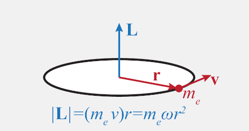
Answer: After discovering his rela-tivistic equations of the new, quan-tum mechanics (Relativistic III), Dirac applied them to the lack of angular momentum, showing how the previously discovered spin exa-ctly covers this difference, and that the matrices of the Pauli spin also enter into the parts of his formulas. Let's look at what follows from free particle first based on Dirac's formulas.

1. Example. Starting from its wave equation along the abscissa:

$$ \psi(x, t) = \mathbf{u}e^{\frac{i}{\hbar}(\mathbf{p}\cdot \mathbf{x} - Et)}, $$

where u = u(E, p) is a vector function of the energy and momentum vector along the abscissa. It does not depend on time and using this we derive the time-independent Dirac equation.

Solution: Substituting into the Dirac equation, we get:

$$ i\hbar\frac{\partial \psi}{\partial t} = -i\hbar c\hat{\alpha}\nabla \psi + \hat{\beta} mc^2\psi, $$ $$ E\mathbf{u}\ e^{\frac{i}{\hbar}(\mathbf{p}\cdot \mathbf{x} - Et)} = -i\hbar c\hat{\alpha}[\nabla \ e^{\mathbf{p}\cdot \mathbf{x} - Et)}] + \hat{\beta} mc^2\mathbf{u} \ e^{\frac{i}{\hbar}(\mathbf{p}\cdot \mathbf{x} - Et)}, $$ $$ E\mathbf{u}\ e^{\frac{i}{\hbar}(\mathbf{p}\cdot \mathbf{x} - Et)} = -i\hbar c\hat{\alpha}[\frac{i}{\hbar}\mathbf{p} \ e^{\frac{i}{\hbar}(\mathbf{p}\cdot \mathbf{x} - Et)}] + \beta mc^2\mathbf{u} \ e^{\frac{i}{\hbar}(\mathbf{p}\cdot \mathbf{x} - Et)}, $$ $$ E\mathbf{u}\ e^{\frac{i}{\hbar}(\mathbf{p}\cdot \mathbf{x} - Et)} = (c\hat{\alpha}\mathbf{p} + \hat{\beta} mc^2)\ e^{\frac{i}{\hbar}(\mathbf{p}\cdot \mathbf{x} - Et)}, $$ $$ E\mathbf{u}(E,\mathbf{p}) = (c\hat{\alpha}\mathbf{p} + \hat{\beta} mc^2)\mathbf{u}(E,\mathbf{p}). $$

It is a time-independent Dirac equation in momentum space. ∎

2. A stationary particle would have momentum p = (p_x, p_y, p_z) = (0, 0, 0). From the above equation we get $E\mathbf{u}(E, 0) = \hat{\beta}mc^2\mathbf{u}(E, 0)$, and when we divide both sides by mc² we get:

$$ \hat{\beta} \mathbf{u}(E,0) = \frac{E}{mc^2}\mathbf{u}(E, 0). $$

This is the characteristic equation $\hat{\beta}\mathbf{u} = \lambda\mathbf{u}$ of the eigenvalue λ = E/mc² and the eigenvector u of the linear operator $\hat{\beta}$. Therefore, we have:

$$ \begin{pmatrix} \hat{I} & 0 \\ 0 & -\hat{I} \end{pmatrix} \begin{pmatrix} \mathbf{u}_a \\ \mathbf{u}_b \end{pmatrix} = \frac{E}{mc^2} \begin{pmatrix} \mathbf{u}_a \\ \mathbf{u}_b \end{pmatrix} $$

from which two equations follow: u_a = λu_a and u_b = -λu_b. In the first, when u_a ≠ 0, then λ = +1, so u_a = (φ₁, φ₂)^⊤ is a column vector with two arbitrary components. In the second, when u_b ≠ 0, then λ = -1, so u_a = (φ₃, φ₄)^⊤ is a column vector with two arbitrary components again. Recall, λ = E/mc².

So, in the first case λ = +1 it will be E = mc² and the energy is positive, of the sign of the mass. In the second case λ = -1 it will be E = -mc² and the energy is negative, of the sign opposite to the mass. These two solutions (λ = ±1) lead to the vectors:

$$ \mathbf{u}_{+} = \begin{pmatrix} \varphi_1 \\ \varphi_2 \\ 0 \\ 0 \end{pmatrix} = \varphi_1\begin{pmatrix} 1 \\ 0 \\ 0 \\ 0 \end{pmatrix} + \varphi_2\begin{pmatrix} 0 \\ 1 \\ 0 \\ 0 \end{pmatrix} = \varphi_1\mathbf{e}_1 + \varphi_2\mathbf{e}_2, $$ $$ \mathbf{u}_{-} = \begin{pmatrix} 0 \\ 0 \\ \varphi_3 \\ \varphi_4 \end{pmatrix} = \varphi_3\begin{pmatrix} 0 \\ 0 \\ 1 \\ 0 \end{pmatrix} + \varphi_4\begin{pmatrix} 0 \\ 0 \\ 0 \\ 1 \end{pmatrix} = \varphi_3\mathbf{e}_3 + \varphi_4\mathbf{e}_4. $$

These are the two eigenvectors for a zero-momentum wave-particle, the solu-tions of the positive and negative energies of the Dirac equation, for the two wave equations:

ψ₊(x, t) = u₊e^-imc²t/ℏ = (φ₁e₁ + φ₂e₂)e^-imc²t/ℏ = ψ₁(x, t) + ψ₂(x, t),
ψ_-(x, t) = u_-e^+imc²t/ℏ = (φ₃e₃ + φ₄e₄)e^+imc²t/ℏ = ψ₃(x, t) + ψ₄(x, t).

Here we have four independent spinor solutions ψ_k, са k = 1, 2, 3, 4. So much for Dirac's stationary particle-wave.

3. Unlike the Klein-Gordon equation, where negative and positive energies go together and lead to energy collapse, in Dirac's they are separate cases, speci-fically the first two E₁ = E₂ = mc² plus the second two E₃ = E₄ = -mc². We can write them as a linear combination in dual forms:

$$ \psi^\dagger(x, t) = \sum_{k=1}^4 \varphi^*_k \mathbf{e}^\dagger_ke^{+\frac{i}{\hbar}E_kt}, \quad \psi(x, t) = \sum_{k=1}^4 \varphi_k \mathbf{e}_ke^{-\frac{i}{\hbar}E_kt}, $$

adjoint (conjugate and transpose of vectors and matrices). We need both to arrive at an expression for the probability density:

$$ \rho(x,t) = \psi^\dagger(x,t)\psi(x,t) = \sum_{j=1}^4\sum_{k=1}^4 \varphi^*_j\varphi_k\mathbf{e}_j^\dagger \mathbf{e}_k e^{\frac{i}{\hbar}(E_j - E_k)t}. $$

Since $\mathbf{e}^*_j\mathbf{e}_k = \delta_{jk}$, which is one only when j = k and zero otherwise, and in addition E_k - E_k = 0 for each k = 1, 2, 3, 4, when we have e⁰ = 1, that is:

$$ \rho(x,t) = \sum_{k=1}^4 \varphi^*_k\varphi_k = |\varphi_1|^2 + |\varphi_2|^2 + |\varphi_3|^2 + |\varphi_4|^2 ≥ 0. $$

Therefore, the Dirac probability density is a non-negative number. Klein had previously derived a quantum mechanical equation that gave both negative energies and probability densities, with physically incorrect solutions.

4. When a particle is moving it has momentum, p ≠ 0, so we calculate:

$$ E\mathbf{u}(E,\mathbf{p}) = (c\hat{\alpha}\mathbf{p} + \hat{\beta} mc^2)\mathbf{u}(E,\mathbf{p}) = $$ $$ = \left(\sum_{k=1}^3 cp_k\hat{\alpha}_k + \hat{\beta}mc^2\right)\mathbf{u}(E,\mathbf{p}) $$ $$ = \left[\begin{pmatrix} 0 & c\sum_{k=1}^3\hat{\sigma}_kp_k \\ c\sum_{k=1}^3\hat{\sigma}_kp_k & 0 \end{pmatrix} + \begin{pmatrix} \hat{I}mc^2 & 0 \\ 0 & -\hat{I}mc^2 \end{pmatrix}\right]\mathbf{u}(E,\mathbf{p}) $$ $$ = \begin{pmatrix} \hat{I}mc^2 & c(\sum_{k=1}^3\hat{\sigma}_kp_k) \\ c(\sum_{k=1}^3\hat{\sigma}_kp_k) & -\hat{I}mc^2 \end{pmatrix} \mathbf{u}(E,\mathbf{p}), $$ $$ E\mathbf{u}(E,\mathbf{p}) = \begin{pmatrix} \hat{I}mc^2 & c(\vec{\sigma}\cdot\mathbf{p}) \\ c(\vec{\sigma}\cdot\mathbf{p}) & -\hat{I}mc^2 \end{pmatrix} \mathbf{u}(E,\mathbf{p}). $$

Here we have used the alpha and sigma matrices explained earlier (Relativistic III, 5) with the notations adapted here. Considering the separation of compon-ents (2), we find:

$$ E\mathbf{u}(E,\mathbf{p}) = \begin{pmatrix} E\mathbf{u}_a \\ E\mathbf{u}_b \end{pmatrix} = \begin{pmatrix} \hat{I}mc^2 & c(\vec{\sigma}\cdot\mathbf{p}) \\ c(\vec{\sigma}\cdot\mathbf{p}) & -\hat{I}mc^2 \end{pmatrix} \begin{pmatrix} \mathbf{u}_a \\ \mathbf{u}_b \end{pmatrix}, $$ $$ \begin{pmatrix} E\mathbf{u}_a \\ E\mathbf{u}_b \end{pmatrix} = \begin{pmatrix} \hat{I}mc^2\mathbf{u}_a + c(\vec{\sigma}\cdot\mathbf{p})\mathbf{u}_b \\ c(\vec{\sigma}\cdot\mathbf{p})\mathbf{u}_a - \hat{I}mc^2\mathbf{u}_b \end{pmatrix}, $$ $$ E\mathbf{u}_a = \hat{I}mc^2\mathbf{u}_a + c(\vec{\sigma}\cdot\mathbf{p}), \quad E\mathbf{u}_b = c(\vec{\sigma}\cdot\mathbf{p})\mathbf{u}_a - \hat{I}mc^2\mathbf{u}_b, $$ $$ \mathbf{u}_a = \frac{c(\vec{\sigma}\cdot\mathbf{p})\mathbf{u}_b}{E - mc^2}, \quad \mathbf{u}_b = \frac{c(\vec{\sigma}\cdot\mathbf{p})\mathbf{u}_a}{E + mc^2}, $$ $$ \mathbf{u}_a = \frac{c(\vec{\sigma}\cdot\mathbf{p})\mathbf{u}_b}{E - mc^2} \frac{c(\vec{\sigma}\cdot\mathbf{p})\mathbf{u}_a}{E + mc^2} \mathbf{u}_a, $$ $$ \hat{I} = \frac{c(\vec{\sigma}\cdot\mathbf{p})\mathbf{u}_b}{E - mc^2} \frac{c(\vec{\sigma}\cdot\mathbf{p})\mathbf{u}_a}{E + mc^2} = \frac{c^2(\vec{\sigma}\cdot\mathbf{p})^2}{E^2 - m^2c^4}. $$

However, by adding matrices and squaring, we find:

$$ (\vec{\sigma}\cdot\mathbf{p})^2 = (\hat{\sigma}_1p_x + \hat{\sigma}_2p_y + \hat{\sigma}_3p_z)^2 = \mathbf{p}\cdot\mathbf{p}\hat{I}, $$

so the previous equality becomes:

$$ \hat{I} = \frac{p^2c^2}{E^2 - m^2c^4}\hat{I}, $$ $$ E^2 = p^2c^2 + m^2c^4. $$

That is the correct relativistic expression for energy.

5. We further verify that $\hat{H}\mathbf{u}_k = E\mathbf{u}_k$, where k ∈ {1, 2, 3, 4}, are the character-istic equations to which the Dirac equation reduces, with only two eigenvalues $E = \pm\sqrt{p^2c^2 + m^2c^4}$ plus sign for k ∈ {1, 2} and minus sign for k ∈ {3, 4} and with the common Dirac Hamiltonian $\hat{H} = c\hat{\alpha}\mathbf{p} + \hat{\beta}mc^2$ and eigenvectors:

$$ \mathbf{u}_1 = N_1\begin{pmatrix} 1 \\ 0 \\ \frac{cp_z}{E+mc^2} \\ \frac{c(p_x + ip_y)}{E + mc^2} \end{pmatrix}, \quad \mathbf{u}_2 = N_2 \begin{pmatrix} 0 \\ 1 \\ \frac{c(p_x - ip_y)}{E + mc^2} \\ \frac{-cp_z}{E+mc^2} \end{pmatrix}, $$ $$ \mathbf{u}_3 = N_3\begin{pmatrix} \frac{cp_z}{E-mc^2} \\ \frac{c(p_x + ip_y)}{E - mc^2} \\ 1 \\ 0 \end{pmatrix}, \quad \mathbf{u}_4 = N_4 \begin{pmatrix} \frac{c(p_x - ip_y)}{E - mc^2} \\ \frac{-cp_z}{E - mc^2} \\ 0 \\ 1 \end{pmatrix}. $$

The check is simply to plug these values ​​into Dirac's equation (4) and see if th-ey agree. To help with these otherwise complex matrix calculations, note that we can work in a standard basis. We do this with the vector u_a = (1, 0)^⊤ so u_a = (0, 1)^⊤, combining with the found u_b to get u₁ and u₂. We derive them from the wave equation:

$$ \psi(x,t) = \begin{pmatrix} \mathbf{u}_a \\ \mathbf{u}_b \end{pmatrix} e^{i(\mathbf{p}\cdot x - Et)/\hbar}. $$

Similarly, we do the reverse, from u_b = (1, 0)^⊤ to u_b = (0, 1)^⊤, combining them with the above u_a to obtain u₃ and u₄ using the wave equation. The constants N_k are arbitrary, and we choose them so that these vectors are unit vectors. So these vectors are orthonormal, i.e. ⟨u_j, u_k ⟩ = δ_jk.

6. Of the four independent solutions to the Dirac equation, the first two, u₁ and u₂, are for particles of positive energy, and the next two, u₃ and u₄, for some negative energies, and it was only around 1930 that he proposed the idea of ​​a Dirac sea. Naturally, all states tend to lower energies, so a spontaneous flow to minus would be a paradox of the theory. He imagined a vacuum like a sea filled with anti-particles, which are fermions and occupy all possible sta-tes. When one of the particles jumps out of such a filling, due to the laws of conservation of energy, momentum, and electric charge, the particle and its hole have opposite signs and the same absolute values. Later, and independe-ntly of Dirac, such an antiparticle, the positron, was indeed discovered by Anderson experimentally.

The notations v₂(E, p) = u₃(-E, -p) and v₁(E, p) = u₄(-E, -p) are introduced for negative energies of the wave function, so we have:

$$ \mathbf{u}_3(E,\mathbf{p}) e^{\frac{i}{\hbar}(\mathbf{p}\cdot\mathbf{x} - Et)} \to \mathbf{v}_2(E,\mathbf{p}) e^{-\frac{i}{\hbar}(\mathbf{p}\cdot\mathbf{x} - Et)}, $$ $$ \mathbf{u}_4(E,\mathbf{p}) e^{\frac{i}{\hbar}(\mathbf{p}\cdot\mathbf{x} - Et)} \to \mathbf{v}_1(E,\mathbf{p}) e^{-\frac{i}{\hbar}(\mathbf{p}\cdot\mathbf{x} - Et)}. $$

Thus we get that the Dirac equation has four solutions of all positive energy, two u₁ and u₂ for particles and two v₂ and v₁ for antiparticles. A new question remains, why there are two such solutions, and not just one. The answer to this leads us to spin.

7. Symmetries, or conservation laws, apply to some quantities (position, mom-entum, energy) that are represented by linear operators, e.g. Â. The expected value of such a quantity is ⟨Â⟩. This is the mean value of its observables taken according to the probability distribution of occurrence. The change in time of this mean value is a function

$$ \frac{dA}{dt} = \frac{d}{dt}\langle \hat{A}\rangle = \frac{i}{\hbar}\langle \psi | [\hat{H}, \hat{A}]| \psi\rangle $$

which is identically equal to zero when for a given observable A, the set of va-lues ​​of its species, the conservation law holds. A special Hamiltonian is Ĥ, the total energy operator. The square brackets define a commutator that measures how much these operators do not commute:

[Ĥ, Â] = ĤÂ - ÂĤ.

Unlike perceptual information, in this information theory, this non-commuta-tivity is a measure of external information (In and Out). It speaks of the prese-nce of an external force with which the  interacts, which distracts it from "in-ertial" motion. Otherwise, when [Ĥ, Â] = 0, then $\frac{d}{dt}\hat{A} ​​= 0$, this means that th-ere is no change in the mean value of the observables (A) over time, and that the conservation law applies to them.

8. Example. Let us apply the commutator of the free particle Hamiltonian from the Schrödinger equation:

$$ -\frac{\hbar^2}{dx^2} \frac{d^2\psi}{dx^2} = E\psi $$

to the circular momentum operator $\hat{L} = \hat{r} \times \hat{p}$.

Solution: We write this Schrödinger equation with operators:

$$ \hat{H}\psi = E\psi, \quad \hat{H} = \frac{\hat{p}^2}{2m}, \quad \hat{p} = -i\hbar \frac{d}{dx}, $$

so we apply this Hamiltonian to the angular momentum:

$$ [\hat{H}, \hat{L}]\psi = [\frac{\hat{p}^2}{2m}, \hat{r}\times\hat{p}]\psi = \frac{\hat{p}^2}{2m}(\hat{r}\times\hat{p})\psi - (\hat{r}\times\hat{p})\frac{\hat{p}^2}{2m} = 0. $$

Therefore, the conservation law applies to angular momentum in relativistic quantum mechanics. ∎

We observe angular momentum in long twirling (gyrate), even strange (Dzha-nibekov), rotations of objects, or orbits (Barycenter) with various proofs of the same law of conservation of rotations. This example is another contribution to such methods, now the Schrödinger equation. Dirac's relativistic equation of the same waves of the quantum world also predicts spin as an addition to it, a phenomenon that was previously observed by measurement and then only ad-ded to other solutions.

9. However, the angular momentum operator, $\hat{L} = \hat{r}\times\hat{p}$, is not commutative with the Hamiltonian, $\hat{H} = c\alpha\cdot\hat{p} + \beta mc^2$, of a free Dirac nonrelativistic qua-ntum particle:

$$ [\hat{H}, \hat{L}] = [c\alpha\hat{p} + \beta mc^2, (\hat{r}\times\hat{p})] = [c\alpha\hat{p}, (\hat{r}\times\hat{p})] \ne 0. $$

Namely, let's break this down into the components of the operator:

$$ [\hat{H}, \hat{L}_x] = [c\alpha_x\hat{p}_x + c\alpha_y\hat{p}_y + c\alpha_z\hat{p}_z, (\hat{y}\hat{p}_z - \hat{z}\hat{p}_y] = $$ $$ = c\alpha_y[\hat{p}_y, \hat{y}]\hat{p}_z - c\alpha_z[\hat{p}_z, \hat{z}]\hat{p}_z = -i\hbar c(\alpha_y\hat{p}_z - \alpha_z\hat{p}_y), $$ $$ [\hat{H}, \hat{L}_x] = -i\hbar c(\alpha\times \hat{p})_x, $$ $$ [\hat{H}, \hat{L}_y] = -i\hbar c(\alpha\times \hat{p})_y, $$ $$ [\hat{H}, \hat{L}_z] = -i\hbar c(\alpha\times \hat{p})_z, $$

and this sums up to:

$$ [\hat{H}, \hat{L}] = -i\hbar c\alpha \times \hat{p} \ne 0. $$

The noncommutativity of the position and momentum operators was used:

$$ [\hat{x}, \hat{p}_x] = [\hat{y}, \hat{p}_y] = [\hat{z}, \hat{p}_z] = i\hbar, $$

which are Heisenberg's uncertainty relations (Impossibility).

10. The change in angular momentum of a non-relativistic quantum free particle with time is not zero, but is constant:

$$ \frac{dL}{dt} = \frac{d}{dt}\langle \hat{L}\rangle = \frac{i}{\hbar}\langle \psi | [\hat{H}, \hat{L}]| \psi\rangle = -i\hbar c(\alpha \times \hat{p}) = \text{const.} $$

which means that (according to my information theory) it is in a constant force field, or (Dirac, officially) that some constant addition that essentially belongs to the particle is omitted in that calculation. That addition is the spin, the physical S the operator Ŝ. The total angular momentum is thus $\hat{J} = \hat{L} + \hat{S}$ and it commutes with the Hamiltonian of the non-relativistic wave equation. The value of the spin is simply the negative specified, $-\frac{dL}{dt}$, so the commuta-tor is zero and the average value of the total momentum Ĵ does not change in time, which means that the conservation law holds for such a particle, which also holds for both its sums $\hat{L}$ and $\hat{S}$. Then from:

$$ [\hat{H}, \hat{S}] = i\hbar c(\alpha\times\hat{p}) $$

we easily find the spin operator:

$$ \hat{S} = \frac{\hbar}{2}\begin{pmatrix} \sigma & 0 \\ 0 & \sigma \end{pmatrix} $$

where sigma can be any of the Pauli matrices:

$$ \sigma_x = \begin{pmatrix} 0 & 1 \\ 1 & 0 \end{pmatrix}, \quad \sigma_y = \begin{pmatrix} 0 & -i \\ i & 0 \end{pmatrix}, \quad \sigma_z = \begin{pmatrix} 1 & 0 \\ 0 & -1 \end{pmatrix} $$

which were hinted at at the beginning (Relativistic III, 4). Let's not forget that this is Dirac's "modest" non-relativistic story about the electron itself.

Honesty » srb

Question: Why do we desire honesty and why is it often absent?

Answer: From my point of view, it's just a very formal story, and some-where between algebra and the the-oretical physical science of lies (still not officially existing).

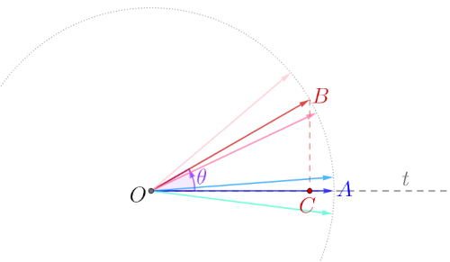
The image on the left represents t one of the possible paths, an imagi-nary flow of reality where at one moment the state A and the state B that we would predict arise. Even knowing almost everything about the state O, because everything is not possi-ble to know due to the assumed uncertainty, it is likely that we would make mistakes in estimating, state $\overrightarrow{OB}$, what will actually happen about state $\overrightarrow{OA}$. Something different could have happened A', A'', ..., which is essentially the assumed uncertainty. But nature does not like equality, so all of her choices are unequal and not necessarily the most probable. The larger the angle θ = ∠(AOB) between the two states, the larger the error in the estimate B, and the shorter the projection, the length |OC| = |OB| cos θ. This results in a smaller "information perception", the scalar product:

$$ \langle A, B \rangle = \overrightarrow{OA} \cdot \overrightarrow{OB} = |OA||OB|\cos\theta. $$

All further stories about "honesty", as far as I'm concerned, revolve around this formula and possibly about (attempted) applications of it in our lives. Here's how.

1. Reality has choices, and that is the lowest level of choice, the backbone of “truth.” In the nature of real events, there is only truth. What we could prove to be untrue by algebra and similar forms would not happen, so I take that ki-nd of “truth” as a standard. It is a die that determines, serves to compare, and verify the notion of “accuracy” of other measures and phenomena, at least as far as this theory is concerned. However, reality, in addition to truthfulness and observability, has the property of permanence. Hence, I consider sustain-ability and interaction as the other two determinants of “truth,” especially in its use.

There are many sayings like “lies have short legs” that speak of the meager re-liability of fictions in general, so it is perhaps more interesting (invisible is) to note that “reality” (so defined) consists of the collective perceptions of oursel-ves and other participants. In the small world of particle physics, particles do not exist until they are observed, measured, or interacted when they are supe-rpositions of multiple states. Only the collapse into one of them, which is an interaction, or the observation by another, does what is reality, which we call a particle, arise. Communications in that micro-world are rare, unlike the almo-st countless in the big world, so we could not notice this phenomenon for cen-turies. For example, the Moon will not disappear when we are not looking at it, because then countless others are looking at it and it is reality.

2. Truth arises through observation. Movements in the cosmos are not only displacements of existing ones (recreations), but also formating (creations) of ever new states and processes. There have been algebraic proofs of the unique-ness of these states since we interpreted reality, phenomena and changes with vectors (Only One). This has the consequence that the question of "real truth" is no longer as clear as formal logic dictates, that on the other hand, the flow of "probability forces" is an effort against the "forces of uncertainty" (new concepts of this theory). The greater the deviation from reality, the greater the angle θ in a given image, the more weight it gains in simulations of truth. In-vention requires greater intellectual effort than remembering the truth. Of course, once it has been invented, the truth is more attractive due to less in-formation in perception, consistent with the principle of minimalism.

3. The difference between creation and created lie space is “vitality”. This is another new term for the addition of fiction to reality when a greater ability to choose arises and with it an addiction to lies (Aquaplaning). Since we can lie, the intellect is fed by it, and then it is drawn into the subsequent attraction of lies. Vitality is that mortal part of a possible living being compared to the im-mortal physical substance, which we compensate for with the ability to model that physical substance, to overcome it (Traits).

This is the secret of "dishonesty", according to this theory. Deceptions are fail-ures of reality and, as in the picture above, require the effort of invention that feeds our intellect (maintains its status quo), and then becomes desirable to others, so the person who lies becomes more popular. Politicians and people who live off the support of many have to lie, in their "pool full of crocodiles", but there is also a trap of disgust after unfulfilled promises, due to the collapse of their "house of cards" (Disgusting). Just as lying is difficult to come by, and created attracts, lies, no matter how popular they are at first, can later be dis-gusting. This is often misunderstood in the sad fate of some politicians, or in the transience of fashion in general.

4. All living biological species lie in one way or another. Deception is such a widespread strategy that organisms use it to survive and reproduce through various methods such as mimicry, camouflage, and generally behavioral tric-ks, and the question of survival arises given the "sand towers" that liars build. Strategies of lying for the sake of lying are weaker than lying for the sake of truth. For example, mathematics uses both ⊤ and ⊥ in the proof of a theorem, in practice we say cheating the cheater, or lying to the liar, possible struggles for the truth.

I suppose that through the sifting process of evolution, aversion to untruth arose, like aversion to rotten food because of possible disease, and we know that it existed even before the discovery of microbes and infections. Similarly, our intuition, i.e. the memory of generations, tells us with a kind of disgust that a life of lies may lead us to ruin. That's why people describing a desired marriage partner will emphasize honesty or sincerity. The best fraudulent society is weaker than the average normal state, because it lags behind reali-ty, which is ultimately the only one that matters.

Balance II » srb

Question: Can you explain this "interesting" connection between honesty with reciprocity and game theory?

Answer: Good or evil are only our experiences that physical nature does not perceive, nor do lies. De-aling with them is lagging behind reality, losing the pace of that race, the game that ultimately counts on-ly for proximity to the truth. This literally means that by wanting to be “good” or “bad”, we easily fall off the rails, we lose reality because of “white lies” (exaggeration in taking things out of context), as well as “black lies” (which we know are untrue). Exaggerating either of these is a reci-pe for failure, but Balancing them can achieve a good middle ground and keep pace with reality.

An example of a white lie is telling a friend that they look great in their clothes when you don't really like them. Also, saying "I'm fine" when you're not, to av-oid further discussion about it, and even censorship by the official media. It has been observed that, for example, monkeys also use deception to take food from weaker colleagues (White and black lies). I believe that these situations have already taught us that tactical (short-term) gain from good or bad beha-vior could be strategic (long-term) loss and vice versa. And here we could add a little formal insight into this knowledge.

1. From the point of view of pure physics, we are unnatural. But when we look a little closer (Honesty, 2) our perception is also a creation, it is not just imagi-nation, and even by passive participation we influence the course of reality at least a little. This is important for explaining the strategies of competition with opponents, among which I will include physical nature itself. It is such a third league (Traits) because it does not see our tricks, when we are its opponents, tamers and builders. Physical nature is blind to lies, and anyone with a little vitality has a good chance of fighting her, although she is indestructible and he is not. He, the one who has more choices, freedom that has its price.

2. Waves are the deepest structure of substance and existence, they add up like vectors and thus they are, often invisible to us, the basis of all other phenome-na. Wavelengths indicate their strength (momentum), and amplitudes visibili-ty (communicativeness). Considering that perception stimulates creation, but the ranges of higher amplitudes are shorter (Wave in Wave), it would seem th-at, metaphorically, the silent one is better than the talkative one. In other wor-ds, the global convergence or tendency of processes towards their inherent st-ate (Hermitian II) is a danger that tends to nullify every achievement of the vital. Therefore, roam freely, wander, but he who remains silent but does not abandon the path of truth also reaches far.

3. Silence that has the effect of mystery awakens the "forces of uncertainty" th-at are the basic drivers of everything, including winning in competition, at lea-st for this theory. If someone constantly jumps, he becomes predictable, read, and a chatterbox, he is left without the magic of surprise that I would put in fi-rst place in the skills of a strategist. In second place is good reading of actions, and in third place is the most important thing from the question posed, which is measured reactions. Every move in the game, be it chess-like (me, then you, then me...) or politics (multidimensional), is a separate problem. However, an honest or sincere attitude towards the problem implies discovering the path to reality in each such situation, and the distance between the mean value of the answer and the truth is a measure of the weakness of the game. Of the two pl-ayers, the one who plays (statistically) weaker loses.

4. In competition with physical substance, we are in a paradoxical situation. It does its work of evading without noticing that it could do otherwise, while we chase it like predators leaping after skillfully eluding prey.

We lie to ourselves not because we have to, but because we want to. Even if we know that an honest and sincere approach to challenges would increase our chances of success tomorrow, we prefer to indulge in the satisfaction of fanta-sy today. The pleasure of the lack of information density of the deception itself in the desire not to decipher it is similar to the attraction of less unexpectedn-ess in the laws, rules, and efficiencies found. We get the first immediately and regret it later, and the opposite is true with the second. The ability to procrast-inate separates strategists from losers.

Present II » srb

Question: Explain to me that unusual concept of "present travel", how do you describe physical reality?

Answer: You've scratched the sur-face, and let's move slowly so we don't get carried away. In physics, superposition is the principle of adding linear systems as vectors, two or more stimuli go with indivi-dual sums into a common effect. The resulting disturbance of the encounter of two or more waves is the algebraic sum of the individual disturbances at that point. It is also the concept of adding particles, atoms, or molecules, and it is true that we ourselves are composed of sums of such. Both of atoms and of superpositions of physical phenomena.

For the sake of clarity, I use the term "physical reality" here as a phenomenon that is permanent, naturally observable and true, contrary to the true goals of this information theory. The other ones, which are locally unstable informati-on are, they disappear as soon as they appear. If information is the true fabric of physical reality (the assumption of this theory), then it flickers with every part and lies on a sea of ​​something that is constantly arising and disappearing in order to maintain itself. It sounds absurd, but it is not contradictory and you will get used to it.

The repeating bits make up reality. Their abstract appearance in the sequence (of ours, the one observing it) over time is that reality, and the fundamental question here is how these details of time become our time flow. To understa-nd this, let us note that “present” can be viewed apart from “duration”. Just as we view the unreal and the real separately. To this part of this theory, we can, for example, add the relativity of simultaneity and quantum uncertainty.

For participants in the movement, the present is not simultaneous (Einstein, 1905), and the uncertainties of time Δt depend on the observed change in ene-rgy ΔE so that ΔE Δt ≥ h (Heisenberg, 1927). Einstein connects simultaneous places with the paths of light, assuming that time stands still at the speed of light, and this “rest” has an uncertainty Δt, with respect to the latter. In other words, a photon appeared and disappeared through one of its oscillations du-ring Δt the time of the observer. While we imagine that a photon travels along the space we are looking at, we can also say that this photon is unique and that it ceased to exist in the same place where it appeared, and was changed by ot-hers along the way. In this way, the past of "reality" is created, while individu-al flashes can only have a Present.

Multiple simultaneous present times, if there are any, superpose to form one of greater energy ΔE and the same shorter time uncertainty Δt ≈ h/ΔE. The long-term indeterminacy (of less energy) overlaps several shorter ones (of greater energy), which means that the lesser energy lasts in the greater, not vice versa, so it makes sense to say that a photon lasts in more of our mome-nts. As in that previous article (Light II), the consequence of all these under-standings is the movement of present times (all larger than photons) at the speed of light in some uncertainty, the surrounding universe. This is actually the shift that makes it seem to us that particles whose time stands still move at the speed of light. Slower-moving particles do not have as much time dilation and a similar estimate is a more complex calculation.

Reality is rushing into the future very quickly. There is a possibility of followi-ng it, but it is practically impossible for vitals (Honesty), as well as for pheno-mena that go to other dimensions of time. Between the two, from a small devi-ation of lies to a complete fallout from the flow of reality, is a large part of my theory, mostly untold.

Overload » srb

Question: I'm not sure what you mean when you say that when we are overinf-ormed, we are misinformed. (Mastery, 4)?

Answer: It seems paradoxical, but such is the nature of information. It is a quantity of uncertainty, and wi-th an overload of unknown news, insight and control of all becomes too much work. Even light is too slow for the large communication synapses in our brain, and artificial intelligence, the text from which you quote the question, has similar limitations.

1. We recognize the universal aversion to uncertainty in the more frequent rea-lization of more probable, less informative outcomes. That is, in short, minim-alism. It supports reality by storing a growing portion of the present's inform-ation in the past, from where it can act, relieving the current present, which then, freed from excess uncertainty, appears more orderly, as if the past were influencing its future. With its increasingly long duration, the present of rea-lity becomes more certain.

2. Space is the accumulator of the past. A star x kilometers away sent light about t = x/300,000 seconds ago, because the speed of light in a vacuum is almost c = 300,000 km/s. The universe tries to preserve its durations with geometric precision so that the present does not lose some of its reality, but global convergence will still do its thing (Just-In-Time) and by disrupting the transmission channel, erase its very distant past and show it to us as the Big Bang. For example, galaxies that are rapidly escaping from us and therefore their clocks tick relatively slowly, we calculate that their Big Bang could have happened much before us (about 13.8 billion years), which is not a problem because we really see it in (for us) its earlier period.

3. Let's ask the same question for a celestial body that is very fast and sudden-ly comes from deep space to fly through the solar system. Have we ever wond-ered why the Big Bang would have occurred at a different time for it from our point of view? While struggling with this puzzle, we suddenly realize that in fact this relative Big Bang did not occur at the same time for objects of differ-ent speeds, that is, that the relative history of the universe did not last the same for everyone. This realization is simply the result of the blurring (noise) of the message through many links in the Markov chain. All messages tend to a specific link in that chain, which then looks like the Big Bang to everyone.

4. As we approach a hill, the hill gets bigger and the surroundings get smaller. We become overinformed by the hill and misinformed. In other ways, this ha-ppens when we peer into the depths of space looking for intelligent life forms, like looking for a needle in a haystack. We become misinformed by the size of the cosmos. A similar thing happens with the noise of a Markov channel, whi-ch increases the transmitted information, thus destroying its message, disin-forming it. This is a degeneration (Degeneration II) that tends to equalize the columns of the composition of the M matrices, which is the Markov chain ge-nerator, that is, the N = Mⁿ matrix, when n → ∞, and the distribution of equa-ls is more uncertain than the selection of privileged ones.

5. Along with information overload leading to disinformation, there is also a spontaneous natural opposite tendency. The first comes because everyone else wants to get rid of it (the excess information), which is why the second arises. They are like an undersea earthquake that triggers a tsunami, which then cra-shes onto the surrounding coasts. A chain of disruptions in which each phase actually only tends to calm down. Examples include some degenerations of so-cial systems that last too long, when an excess of external uncertainty affects the reorganization, or vice versa, if due to great internal uncertainty the syst-em breaks up into smaller, more distinct communities.

6. The Roman Republic, for example, lasted from 509 BC to 27 BC. Its end was a period of political instability and social unrest, and civil wars due to expansi-on, corruption, and the changing nature of the army. After the fall of the Rom-an Kingdom, the Roman Empire was established, which is traditionally mark-ed in 27 BC when Octavian was given the title of Augustus. The Western Rom-an Empire officially collapsed in 476 AD due to corruption, political instabili-ty, economic problems, and external pressures such as invasions. In detail, this blanket assessment would lead to the above, I say this because of mathe-matical certainty and not because of any knowledge of history on my part.

Amorphous II » srb

Question: Again, about that "illusion" of the beginning of the cosmos, how is it possible that after the beginning 13.8 billion years ago, we see the growth of an "amorphous state" into a more "organized" one today?

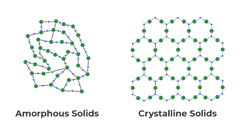
Answer: I think I understand the question, because a similar probl-em has been bothering me for a lo-ng time. We all observe a hot cosm-ic soup growing thinner and cooler, crystallizing into mass, then into atoms, celestial bodies and galaxi-es, and then into various other phe-nomena, "forgetting" their origins. The puzzle is, I paraphrase, wheth-er these forms are real or fictitious.

1. In that range, where you are depends on what you are. Namely, outside of gravity, the flow of time is faster and the gap between the distant vacuum and the celestial bodies, or their "nows", grows. The vacuum traces the future, ma-king matter certain, and a body that would be in between, and whose time has a speed between those two, goes towards the slower one. We say it falls gravit-ationally, and here's why.

A planet near a body partially slows down time compared to places far from the field, and additionally slows down time for itself and its surroundings. Th-is makes the time of a given place with the body slower than the time of the pl-ace itself, that is, the time of the body lags behind the planetary environment. The planet approaches the body, because in each closer position the same pr-ocess is repeated.

The variations of the initial boiling soup could have developed in any other way, forming physically different universes, so that the priority for all such remains the tendency towards more probable states. This is the requirement of my theory, that spontaneous development tends towards less informative, which means variations, and gravity succeeds in this.

2. Once the development of the amorphous state into one of the probable pro-cesses begins, there is no turning back. Global convergence begins, the adapt-ation of those present to similar experiences that are never the same, but bor-ing and less informative. The nature of that single time flow will not allow pa-rticipants to observe large jumps, incredible deviations in situations of large numbers. So subjects in very different events (space-time) will experience a similar universe. From a great distance, or in the vast majority of cases, phe-nomena viewed flow smoothly, and it is only in the micro-world that various relative leaps occur more significantly, creating unexpected things for them.

The Information Perceptions a⋅b = ab cos φ grows by adaptation, because the angle φ = ∠(a, b) then decreases and the cosine increases, if the intensities of the states a = |a| and b = |b| remain the same. This is Internal information of the coupling of two subjects and indicates the possibility (optional) of their co-mmunication, states a and b, which appropriates their attention and to that extent separates it from the outside world. Hence, the adaptation of some may be their alienation from others.

3. Laws are a way to achieve both diversity and predictability, to avoid homo-geneous distributions (i.e. maximum information along a limited interval of random values), without unexpectedness. This is an opportunity that should not be missed by any of the initial developments of the universe and subsequ-ent sequels, if they are based on the assumptions of such a theory, for examp-le, on the objectivity of chance.

I remind you, a certain event here has a probability of 1 and an impossible eve-nt has a probability of 0, although mathematics does not consider these extre-mes to be "coincidences". Consistently, theorems, and even physical laws, are treated here as information, as quantities of uncertainty of quantum packets, the product of changed energy ΔE for time Δt, unlimited duration (Δt → ∞) and zero energy (ΔE → 0). Their obligation comes from the attraction of a sl-ower flow of time, for those subjects who recognize them.

4. It turns out that in theories like this, by accepting objective randomness as a universal principle, the universe becomes specialized. By tending to filter out untruths, transient states, and unobservable phenomena, it actually separates truths and permanent phenomena that can be mutually observed. It drags be-hind it traces of the past due to the weakening of the uncertainty of the prese-nt, sinks into ever greater regularities, and groups itself around independent truths, axioms. In this way, it becomes isolated from alternative developmen-ts, like an archipelago of islands.

The very possibility of alternative developments of the universe is the answer to the above question. Theoretically, there is no single "reality", therefore the more difficult question is why some current reality would be unique to the cu-rrent participants. We know that in ours, every subject is unique. Moreover, according to the laws given to us, the very beginning of all development is a kind of "illusion", albeit so strong that we cannot overcome it with any expe-riments or even with logical reasoning.

Whirligig » srb

Question: Please explain to me the physical properties of a spinner (Coupling, p. 182)?

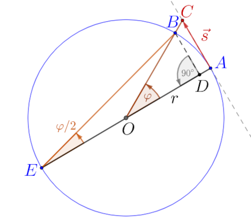
Answer: A peripheral angle ∠AEB, marked φ/2 in the figure on the ri-ght, over the chord AB of the circle with center O and radius:

r = OA = OB = OE

is equal to the angle between the tangent and the chord ∠CAB and is twice the central ∠AOB = φ over the same chord. That's from geo-metry.

Namely, the triangle OBE has equal legs, so at their base they have equ-al angles ∠EBO = ∠OEB = φ/2. However, the exterior angle of the triangle is equal to the sum of its two non-adjacent interior angles, so ∠AOB = ∠EBO + ∠OEB = φ. Hence ∠EBA = 90°, because the peripheral angle over the diame-ter is right because the central angle over the diameter is ∠AOE = 180°. Fin-ally, the angles with perpendicular legs AB ⊥ BE and CA ⊥ AE are equal, so ∠CAB = ∠AEB = φ/2.

1. The circle rotates uniformly, with a constant angular velocity ω, which mea-ns that for equal time intervals Δt the radius r describes equal angles, say OA → OB when it describes an angle φ = ω Δt. The point A moves with a constant velocity v to the position B along an arc of length AB = v Δt. Then it will over-come the acceleration a with which it can cover the path $AD = \frac12 a\Delta t^2$. All points of the circle are not inertial, because they leave tangents like A → C.

For very short time durations Δt → 0, infinitesimal, the arc and the length AB can be considered equal. Then the proportion AC : AD = AE : AB holds, beca-use the angles with parallel sides CA = DB are equal ∠CAB = ∠DBA, but right triangles are also similar ABD ∼ AEB, so we have:

$$ AB : AD = AE : AB, $$ $$ AB^2 = AD\cdot AE. $$

From the previous we now easily calculate:

$$ (v \Delta t)^2 = (\frac12 a\Delta t^2)\cdot(2r), $$ $$ a = \frac{v^2}{r} = r\omega^2, \quad F = mr\omega^2, $$

where the centrifugal force F = ma is equal to the product of the mass m of a given point on the circle and the acceleration mentioned. It pulls the material point A away from O, the center of the circle.

2. To achieve this centrifugal force, the same amount of force is needed to mo-ve the material circle (top, wheel, circular platform); precisely speaking, a for-ce is needed to give it such an initial momentum:

p = mv = mrω.

Тorque, or moment of force $\vec{\tau} = \vec{r}\times \vec{F}$ is a vector of magnitude τ = rF sin θ with an angle θ between the directions of the lever and the force, and the dir-ection of the axis of rotation. This is the force of an object in rotation about an axis and corresponds to the role of a force in rectilinear motion, except that it is perpendicular to the plane of the directions of the lever ($\vec{\tau} \perp \vec{r}$) and the for-ce ($\vec{\tau} \perp \vec{F}$). We note the analogies:

$$ p = mv, \quad L = I\omega, $$ $$ F = \frac{dp}{dt}, \quad \tau = \frac{dL}{dt}. $$

Linear acceleration is $a = \dot{v}$ and rotational acceleration is $\alpha = \dot{\omega}$ and consequ-ently $\tau = I\alpha$. The angular momentum vector of a particle is $\vec{L} = \vec{r}\times\vec{p}$ and, in addition, the moment of inertia is I, and ω is the orbital angular velocity. This is in the development of mathematical physics, and it could have been achiev-ed in a different way.

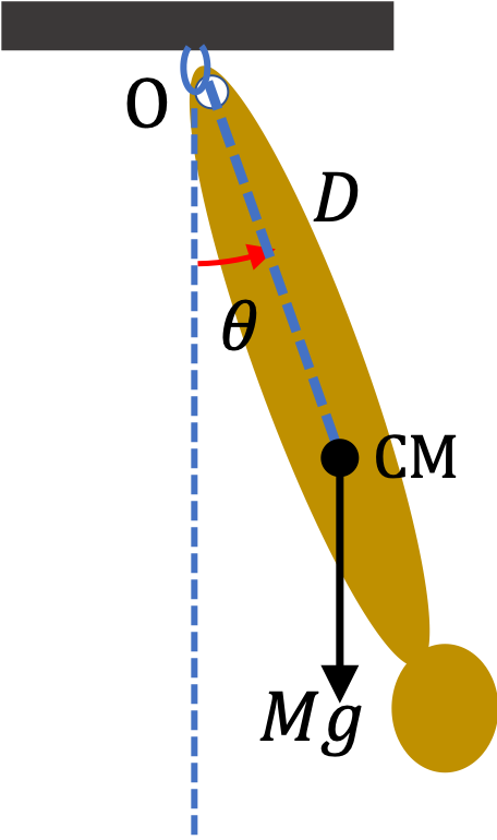
3. In the figure on the left is a physical pendulum. It is any rigid object that swings left and right und-er O, a fixed point of suspension. We distinguish it from the idealized simple pendulum of a point with a mass on a string (Line up). Its motion depends on the mass distribution so the moment of inertia (I) becoming an important factor along with its mass (M), distance (D) to the center of mass (CM), and acceleration due to gravity (g). For small angles (θ), deviations from the vertical and the axis of equilibrium, its oscillation periods (T) can be calculated using the formula:

$$ T = 2\pi\sqrt{\frac{I}{MgD}}. $$

These oscillation periods do not depend on the initial deflection, but they are calculated for small deflections, angles sin θ ≈ θ radians.

4. The image on the right has a link with the orbital velocity:

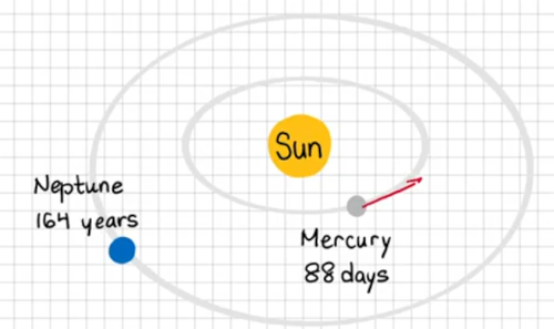
$$ v = \frac{2\pi r}{T} = 29.8 \ \text{km/s} $$

the Earth, with a radius r of 150 million kilometers, orbits the Sun with a period T = 1 year. This is a general formula and is obvious, because the circumference of a circle with radius r is 2πr divided by the elapsed time T gives the orbital velo-city v. A more complex calculation will relate these quantities to the mass of the center of gravity.

As the Earth of mass m orbits the much larger mass M of the Sun, and the ce-ntrifugal force is equal to the gravitational ma = Mg, the mass of the Sun will be:

$$ \frac{mv^2}{r} = G\frac{mM}{r^2}, $$ $$ M = \frac{rv^2}{G} = 2 \times 10^{30} \ \text{kg}. $$

The radius of the Earth's orbit r = 1.5×10¹¹ m, and G = 6.67×10^-11 m³ kg^-1 s^-2 is the gravitational constant. These are also general formulas, applicable to all planets of the solar system and their satellites. Space orbits are universal phe-nomena that take on parts of the energy of bodies.

5. Finally, it can be said that this is why we have the spin of elementary partic-les. Because motion is relative and it is equally true that we are all at rest and kinetic energies are a matter of the environment, hence we have energies rela-tive to other bodies. Then, our reality is how everyone else sees us (that is the insight of this theory), which means that we reduce elementary particles to th-eir spin as well. Therefore, virtual photons (temporary, invisible particles that mediate the electromagnetic force by exchanging between charged particles) are only real through interaction, when they acquire spin (±1).

Fulfill » srb

Question: Can (this) information theory explain the “Double Slit” experiment?

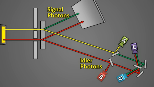
Answer: Yes, of course, I will try to repeat the most important things, but after you watch such a video on the left.

A virtual particle is realized only af-ter observation (interaction) with at least one reality, because reality is an observable, permanent and true phenomenon. Previously, it does not have a real, say, spin or momentum so that it can be radiated without los-ses of these quantities from its source. Secondly, if a particle (photon) moves at the speed of light, there is no flow of time, all positions on its path are sim-ultaneous to it.

1. Retrocausality is a reverse causality. It is a phenomenon that precedes a ca-use, which means that a later event can affect an earlier one. These findings come from quantum mechanics, phenomena such as quantum entanglement, but which we consider here for now as the coupling of “different” events that are otherwise simultaneous in themselves. This "reverse causality" manages to last up to several femtoseconds ( 1 fs = 10^-15 s), which is still too much for the gravitational time deceleration of the operator in the experiment (say m = 100 kg), which at a meter distance would be of the order of Gm/c² ≈ 10^-25 s. Also this multiplied by the tons of the object is still not enough and I leave the qu-estion of such retrocausality of these small particles open.

Namely, taking only the mass of the human body and the time delay due to th-at small gravity, even smaller particles are in the future opposite the operator. But, since that is not enough, I also take into account the weight of the surro-unding equipment, the floor, the walls of the building, then the delay from re-ading the measurement results (limitation of the speed of light), but I do not delve into the measurement technique and cannot say "that's it". Moreover, I am not sure that these measurements are superbly interpreted, nor that gravi-tational delay could be the exclusive cause of the alleged retrocausality. Other-wise, this theory postulates the randomness of the micro world and, therefore, their short occasional walks into the past.

2. BBO crystal is a nonlinear optical crystal made of beta barium borate, and is otherwise valued for its ability to efficiently convert laser light into different frequencies. In the image above on the left, it is inserted behind two holes th-rough which light passes (yellow and red lines) which then splits into two pat-hs (green-yellow and red-red), of which the upper ones (Signal photons) are signals that will (not) interfere on the upper curtain, and the lower ones (Idler photons) go further to curtains A and B which will notice them, or to curtains C and D which mix them so that we cannot know which of the photons passed through which of the initial holes.

What happens in that experiment, simply put, seems to be at the foundation of this theory. Reality defines perception, also duration and truthfulness due to which the collapse of the superposition into a particle is always a continuation of some such reality that will maintain the given quantity. In this way, the se-parated yellow photon goes down as a probability distribution (superposition) and becomes the outcome at the place A, which is why its upper arm is also a particle, although the path to A is further, the lower path, the realization after the signal photon. For this light they are simultaneous, and for us retrocausal.

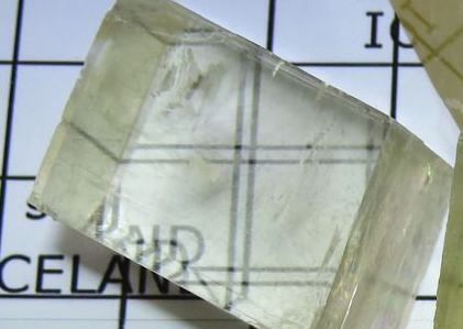
3. Similar to the BBO crystal, calci-te, pictured on the right, also splits light into two streams. We call this phenomenon double refraction or birefringence. Calcite seems to co-ntain materials with different intri-nsic refractive indices that depend on the position between the crystal lattice and the light that falls on it. The important point here is to dis-cuss that such crystals do not split single photons into two photons, but rather direct light waves into two streams. Otherwise, we would have a photon of sp-in ±1 at the input, and two such at the output — which is an impossible calcu-lation.

Calcite is cheaper than BBO crystals and therefore more suitable for improvi-sing the described experiment in the upper left image using small lasers. It is not easy to achieve such a clear retrocausality that would be extremely convin-cing, and on top of that there is the previous remark that we are dealing with different photons. Two go in two directions, and their two streams of different parts of light blur the picture. This does not concern the basic double-slit exp-eriment, but only doubts about the retrocausality described above.

4. An electron is a superposition of possibilities until the first measurement when it collapses into a single outcome that turns out to be a particle. This is the current description of the interpretation of quantum mechanics, which was also advocated by Heisenberg (1927). In the “double slit” experiment, wh-ere electrons are directed one by one, the points of their impact on a screen are stored in a wave pattern of light and dark stripes typical of interference and diffraction. The amplitudes are expressions of the probability of intera-ction (the surface can also let these small particles through) and the wavelen-gths are expressions of momentum. So, before the interaction with the screen, the “electron” is a probability wave, and the imprint of the electron on the sc-reen is the collapse of the “probability wave”. In this way, the story of alleged retrocausality, the interference of electrons arriving at different times, is avoided.

Wherever a wave sphere is “observed,” it will collapse into one outcome, which is its particle. Similar to metamorphoses in biology, interactions will “excrete” waves into particles that continue to live reality. Little of the sphere remains for the second opening, if that communication occurs at the first, and the im-age on the screen behind it is also changed by these “observations.” There is not much difference between the informatics view and the official explanation of the double slit experiment, and I consider this to be confirmation of this theory.

Collapse III » srb

Question: What is the "collapse" of the wave function?

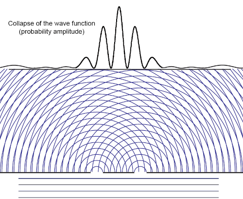
Answer: If you accept the idea of ​​objective randomness, the interpr-etation of superposition and collap-se becomes like, say, the interpreta-tion of a probability distribution against the realization of a random outcome. Noting that in the above distribution there is a probability that none of the outcomes will oc-cur. Otherwise, the collapse of the wave function will remain one of the greatest secrets of quantum mechanics; according to some authors, its only real mystery.

1. The image above on the left shows waves that encounter two openings from below, beyond which they continue to spread in concentric circles. Their inter-sections are "phantom" particles (Arrows), that is, material points that aband-on inertial motion in favor of moving along hyperbolas. These points, interse-ctions of circles, accumulate on the screen above in alternately stronger and weaker diffraction lines that correspond to the interference amplitudes. The amplitudes are increasing expressions of the probability of interaction (with the screen) that are added up by the crossing of the waves, and the waveleng-ths are decreasing expressions of the momentum.

2. Let us label the two narrow openings in the above figure as I₁ and I₂, respe-ctively. If one opening were closed, there would be no interference; it requires more than one wave (Quantum Mechanics, p. 63). Let A₁(I₁) and A₂(I₂) be the amplitudes of the two waves that passed through the openings. At the points of their interference, the amplitude is A = A₁ + A₂. According to the Born's ru-le, the interaction probability of this aggregate output is P(I) = |A|² = A^*A. In quantum mechanics, amplitudes can be complex numbers, and A^* is the com-plex conjugate of A.

3. Let's be more precise. We have a complex number A = a + ib whose real and imaginary parts Re(A) = a and Im(A) = b are both real numbers, with i² = -1 imaginary unit. Then its conjugate is A^* = a - ib. Let I_k denote the passage of a wave through an opening k ∈ {1, 2}. In addition, by multiplying complex num-bers we find for the total amplitude:

|A|² = |A₁ + A₂|² = (A₁ + A₂)^*(A₁ + A₂) =
= A₁^*A₁ + A₁^*A₂ + A₂^*A₁ + A₂^*A₂
= |A₁|² + |A₂|² + 2 Re(A₁^*A₂),

where is:

|A₁|² = a₁² + b₁²,     |A₂|² = a₂² + b₂²,
A₁^*A₂ = (a₁ - ib₁)(a₂ + ib₂) = (a₁a₂ + b₁b₂) + i(a₁b₂ - b₁a₂),
Re(A₁^*A₂) = a₁a₂ + b₁b₂.

The probability of the cumulative interaction is thus:

P(I) = |A₁|² + |A₂|² + 2 Re(A₁^*A₂).

The amplitudes A₁ and A₂ change with time and depending on the location on the screen. They form a maximum to the cancellation of the sum wave, and af-fect the probability of interaction with the screen and the formation of the dif-fraction image.

4. A more careful analysis in continuation of the previous one reveals:

P(I) = (a₁ + a₂)² + (b₁ + b₂)².

The amplitudes of the waves are summed by summing the real and imaginary parts separately to find the interaction probabilities in the same Born rule. When we have the distance between the wave slits (an integer multiple) of the wavelength, since the amplitudes change direction as sinusoids, going up and down, they will be in equal phases at the exit of the slit.

When the apertures are encountered by co-directional amplitudes, the inter-section of concentric circles gives higher probabilities. The lines of the afore-mentioned hyperbolas (Bundle) of the intersection of the output waves that end in bright points (E_k) of the screen contain the highest probabilities, and between them would be the hyperbolas of the lowest probabilities and the darker stripes on the upper screen of the given image. Thus, the above pro-bability becomes logical, and this mathematical check, in addition to confi-rming the previous estimates, opens the way for some more.

5. Tossing a (fair) coin, with probability p of "tails" and probability q of "hea-ds", and some small probability r that neither of the two will come up, so that the sum of all three non-negative numbers is one, is an example that better re-presents superposition. Collapse does not have to occur with the third of the probabilities. Nevertheless, Shannon's information:

S = -p ln p - q ln q - r ln r

after the coin toss (collapse) is exactly equal to the amount of uncertainty before the toss (superposition). In coin practice, because r → 0, it will be:

$$ \lim_{r\to 0} r\ln r = \lim_{r\to 0} \frac{\ln r}{\frac{1}{r}} = \lim_{r\to 0} \frac{(\ln r)'}{(\frac{1}{r})'} = \lim_{r\to 0} \frac{\frac{1}{r}}{-\frac{1}{r^2}} = \lim_{r\to 0}(-r) = 0. $$

The limit calculation uses L'Hôpital's rule. When the third Shannon infor-mation sum is zero and the coin is fair p = q = 1/2, then:

$$ S = -\frac12\ln\frac12 - \frac12\ln\frac12 = \frac12\ln 2 + \frac12\ln 2 = \ln 2 \approx 0.69 $$

It is analogous to distributions (superpositions) with multiple outcomes. That is, when the interference collapse occurs (the intersection points of the circl-es), the delivery of all the uncertainty of the superposition of both circles occ-urs. Those two waves in the intersection after the aperture collapse into one particle, at one place on the screen, which was actually one wave before the aperture.

Amplitude » srb

Question: Why are amplitudes complex numbers?

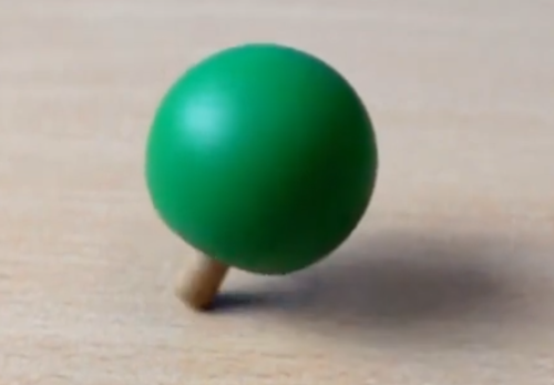
Answer: First, we notice how we “stand on the shoulders of giants” (in Newton’s phrase, 1687), who have climbed truths in solid buil-dings, rejecting lies. So far, we kn-ow that we are a structure of atoms and molecules, then states, then processes as an interpretation of vectors. The image on the right is a link to a video about a Chinese spi-nning top that may reveal the deep-er nature of vectors in precession.

1. We learn about vectors in school, for example, by summing the speed of a boat $\vec{v}_1 = (v_{1x}, v_{1y})$ on the surface of a calm river with $\vec{v}_2 = (v_{2x}, v_{2y})$, the speed of river, by summing it into the speed vector $\vec{v} = \vec{v}_1 + \vec{v}_2 = (v_x, v_y)$ of the boat relative to the shore, where each component of the sum is obtained as the sum of the corresponding components, here we have $v_x = v_{1x} + v_{2x}$ and $v_y = v_{1y} + v_{2y}$. We also add forces in this way, by adding equal directions ob-taining the diagonals of the parallelogram of forces. It is important that the components of the vector lie along independent directions, of everything that can be added. Thus, a particle with momentum $\vec{u}$ and mass $m$ can be treated as a vector sum of the same $(\vec{u}, m) = (\vec{u}_1, m_1) + (\vec{u}_2, m_2)$. There is also the concept of "reality" to distinguish between sustainable and unsustainable phenomena.

2. The states of the system are "ordinary" vectors, such as the aforementioned $\vec{v}$, which in the case of macro-systems can have a huge number of components, or be determined using differential equations, integrals, or their linear sums (which we add as vectors, component by component). These components are independent in such a way that adding one does not affect the sum of the oth-ers, and this is the simplicity of vector calculus. Therefore, vectors also consist of linear processes, such as $\hat{T}$, which in a certain coordinate system will be the matrix T.

In vector algebra, the characteristic equation is very important, $\hat{T}\vec{v} = λ\vec{v}$, wh-ere the operator $\hat{T}$ does not change the direction of its eigenvector $\vec{v}$ but only multiplies its intensity by the eigenvalue λ, which is a scalar (real or complex number). There are as many independent eigenvectors of a given operator as its dimension, which are as many components as that operator written as a vector, $\hat{T}[\vec{v}_1, \vec{v}_2, ..., \vec{v}_n]$ would have, here n = 1, 2, 3, ... They are all solutions of the same characteristic equation, $\hat{T}\vec{v}_k = \lambda_k\vec{v}_k$, for k = 1, 2, ..., n, of the given operator. In quantum mechanics, for the eigenvectors $\vec{v}$ we choose observables (physically measurable quantities), and the eigenvalues ​​$\lambda$ are real numbers. Here's how we find the operator knowing the observable.

3. Example. Given two orthonormal observables, $\|\vec{v}_1\| = \|\vec{v}_2\| = 1$ and $\langle\vec{v}_1, \vec{v}_2\rangle = 0$, in some coordinate system:

$$ \vec{v}_1 = \frac{1}{\sqrt{2}} \begin{pmatrix} 1 \\ i \end{pmatrix}, \quad \vec{v}_2 = \frac{1}{\sqrt{2}} \begin{pmatrix} i \\ 1 \end{pmatrix}, $$

with the corresponding eigenvalues, respectively λ₁ = 2 and λ₂ = 1. Let us find the matrix T of the linear operator $\hat{T}$ of the process to which they belong.

Solution: We form an auxiliary matrix $P[\vec{v}_1, \vec{v}_2]$ of these eigenvectors and its inverse matrix P^-1 = P^†. At the same time, it is adjoint, because the vectors are orthonormal, so we have:

$$ P = \frac{1}{\sqrt{2}} \begin{pmatrix} 1 & i \\ i & 1 \end{pmatrix}, \quad P^{-1} = \frac{1}{\sqrt{2}} \begin{pmatrix} 1 & -i \\ -i & 1 \end{pmatrix}. $$

In the sandwich of the product between them, we put the diagonal matrix D[λ₁, λ₂] and here we have the matrix T of the required operator $\hat{T}$:

$$ T = PDP^{-1} = \frac{1}{\sqrt{2}} \begin{pmatrix} 1 & i \\ i & 1 \end{pmatrix} \begin{pmatrix} 2 & 0 \\ 0 & 1 \end{pmatrix} \frac{1}{\sqrt{2}} \begin{pmatrix} 1 & -i \\ -i & 1 \end{pmatrix} = \frac12\begin{pmatrix} 3 & -i \\ i & 3 \end{pmatrix} $$

written in the coordinate system of given vectors. ∎

Verification yields $T\vec{v}_1 = 2\vec{v}_1$ and $T\vec{v}_2 = 1\vec{v}_2$, as they should be. Note that this matrix is ​​Hermitian, because such matrices have real eigenvalues ​​(λ), but they do not necessarily have real vector coefficients.

4. The eigenvectors $\vec{v}_k$, in example (3) of index k ∈ {1, 2}, span some vector space of states and the changes that the operator $\hat{T}$ can make to them, which we could consider further. In general, this state is of the form:

$$ \vec{x} = \xi_1\vec{v}_1 + \xi_2\vec{v}_2 + ..., \quad \|\xi_1\|^2 + \|\xi_2\|^2 + ... = 1, $$

with amplitudes ξ₁, ξ₂, ... ∈ ℂ which can be complex numbers, and whose squ-ares of the modulus of the probability of finding are observable during measu-rement. As the states are calculated after the measurement, the possible prob-abilities (say ∥ξ₃∥² > 0) that the measurement could have been unsuccessful, i.e. that this interaction did not have to occur, are overlooked.

In eigenvector coordinate systems, we also write the above arbitrary vectors in bold x = (ξ₁, ξ₂, ...)^⊤, with the emphasis (⊤, transpose) that they are column-matrices (contravariant) and omitting the arrows above. However, we also use plain italics x = (ξ_k) with only the general term marked, when we know what we are working with.

5. Let A ∈ {ξ₁, ξ₂, ..., ξ_n} be some of the n = 1, 2, 3, ... observables realized in the measurement. If it were the amplitude of the superposition of, say, three similar particle-waves A = A₁ + A₂ + A₃, then let us calculate the probability of finding the collective observable using the individual ones contained in it:

P(A) = |A|² = A^*A =
= (A₁^* + A₂^* + A₃^*)(A₁ + A₂ + A₃)
= [(a₁ - ib₁) + (a₂ - ib₂) + (a₃ - ib₃)][(a₁ + ib₁) + (a₂ + ib₂) + (a₃ + ib₃)]
= [(a₁ + a₂ + a₃) - i(b₁ + b₂ + b₃)][(a₁ + a₂ + a₃) + i(b₁ + b₂ + b₃)],

where I use the notation from the previous answer (A = a + ib, where a, b ∈ ℝ with the imaginary unit i² = -1), but I go the other way. We get:

P(A) = (a₁ + a₂ + a₃)² + (b₁ + b₂ + b₃)².

From this, the interaction probability is the square of the sum of the real amp-litudes plus the square of the sum of the imaginary ones. It is obvious that the same holds in general for any number of substitution sums:

$$ P(A) = (\sum_k a_k)^2 + (\sum_k b_k)^2, $$

so since in the macro-world we do not see the sums of these b-terms, it could be that they disappear due to the law of large numbers of probability theory. In the micro-world, imaginary b-sums of amplitudes may remain to testify to increased uncertainty, especially for understanding bypassing and as a measu-re of the absence of interaction, but in principle we can also reduce or compli-cate quantum mechanics to work without them.

Еxemption » srb

Question: How do you think quantum mechanics is possible without complex numbers?

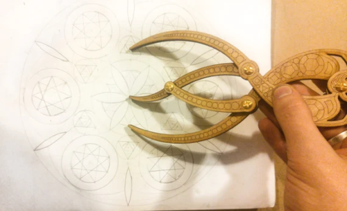
Answer: Just as our ancestors co-uld live without knowledge of ato-ms and molecules. Also, you can perform many geometric constru-ctions with just a compass and a straightedge without division, giv-ing up the convenience of working with various other auxiliary tools. This is just one aspect of the, per-haps now undiscovered, possibili-ties of working with quanta.

The second possibility lies in alternative theories that have yet to be discover-ed. Who would have thought in Euclid's time that his geometry could be equ-ally explored using coordinate systems and equations, or that the ratio of the circumference to the diameter of a circle (the number π ≈ 3.14...) could be ca-lculated from probability theory (Buffon's needle). Namely, unlike untruths, veracities are "only one" in the sense that they are true in different exact con-texts, so even today's quantum mechanics (if it is a correct theory) could tom-orrow be presented in a very different concept.

1. For a unitary operator, $\hat{I}\vec{x} = \vec{x}$, every vector $\vec{x}$ (of a given dimension) is an eigenvector, including those with complex coefficients. For example, $\hat{I}\vec{v}_1 = \vec{v}_1$ and $\hat{I}\vec{v}_2 = \vec{v}_2$, where in a 2-dimensional space this operator has the next unit matrix:

$$ I = \begin{pmatrix} 1 & 0 \\ 0 & 1 \end{pmatrix}, \quad \vec{v}_1 = \begin{pmatrix} 1 \\ i \end{pmatrix}, \quad \vec{v}_2 = \begin{pmatrix} 1 \\ -i \end{pmatrix}. $$

These vectors are also perpendicular, because:

$$ \langle \vec{v}_1, \vec{v}_2\rangle = \begin{pmatrix} 1 & -i \end{pmatrix} \begin{pmatrix} 1 \\ -i \end{pmatrix} = 1 - 1 = 0. $$

However, they are not normed:

$$ \langle \vec{v}_1, \vec{v}_1\rangle = \begin{pmatrix} 1 & -i \end{pmatrix} \begin{pmatrix} 1 \\ i \end{pmatrix} = 1 + 1 = 2, $$ $$ \langle \vec{v}_2, \vec{v}_2\rangle = \begin{pmatrix} 1 & i \end{pmatrix} \begin{pmatrix} 1 \\ -i \end{pmatrix} = 1 + 1 = 2. $$

To make them unitary, divide each by √2. Then, with $\vec{u}_1 = \vec{v}_1/\sqrt{2}$ and $\vec{u}_2$ = $\vec{v}_2/\sqrt{2}$, you will have one orthonormed basis of then 2-dimensional vector space. Linear operators for which each vector is an eigenvector exist only in the case of a scalar (α) multiple of the unit operator αÎ.

2. Except for scalar multiples of the unit operator, the eigenvectors of the Hermitian matrix M = A + iB, separated into two real matrices A and B, are real when the eigenvector v is in the null space B, i.e. if Bv = 0.

Namely, from Mv = v it follows (A + iB)v = v, then Av + iBv = v, so by sepa-rating the real from the imaginary part from this one characteristic equation, we obtain two Av = v and Bv = 0. And that's it, the vector v is from the null space of such a matrix B, which means it is orthogonal to all its columns.

Otherwise, the null space of a matrix B is the set of all vectors x that satisfy the equation Bx = 0. This means that the null space contains all vectors (those th-at do not contain all zero components) that are mapped to the null vector (wh-ose all components are zero) by the matrix.

3. A Hermitian matrix M always has real eigenvalues ​​λ, such that the characte-ristic equation Mv = λv holds. Not all of its eigenvectors (v) need be real. Ho-wever, when the matrix is ​​not Hermitian, as in the following unusual example:

$$ N = \begin{pmatrix} 4 & 1 - i & 0 \\ 1-i & 4 & 0 \\ 0 & 0 & 3 \end{pmatrix}. $$

Non-Hermitian matrix N (N^† ≠ N) has complex eigenvalues ​​λ₁ = 3, λ₂ = 3 + i and λ₃ = 5 - i, but real corresponding eigenvectors, respectively:

$$ v_1 = \begin{pmatrix} 0 \\ 0 \\ 1 \end{pmatrix}, \quad v_2 = \begin{pmatrix} -1 \\ 1 \\ 0 \end{pmatrix}, \quad v_3 = \begin{pmatrix} 1 \\ 1 \\ 0 \end{pmatrix}. $$

It is easy to check by directly multiplying Nv_k = λ_kv_k for k ∈ {1, 2, 3}.

4. It follows from (2) that the only complex Hermitian matrices with all real eigenvectors are those that are themselves real symmetric matrices. When a Hermitian matrix also has complex elements, at least one of its eigenvectors will be complex, it cannot be expressed as a scalar multiple of a non-zero real vector. This is an interpretation of the given condition (2), that all eigenvecto-rs will be real when the imaginary part of the matrix is ​​the zero matrix.

For example, the following real symmetric 2×2 matrix is ​​a special case of a "complex" Hermitian matrix, it has no imaginary parts:

$$ A = \begin{pmatrix} 2 & 1 \\ 1 & 2 \end{pmatrix}, $$

has real eigenvalues ​​3 and 1, with the corresponding eigenvectors (1, 1)^⊤ and (1, -1)^⊤ both real. However, the non-real Hermitian matrix iB with eigenvector v, where:

$$ B = \begin{pmatrix} 0 & 1 \\ -1 & 0 \end{pmatrix}, \quad v = \begin{pmatrix} \alpha \\ \beta \end{pmatrix}, $$

with the condition Bv = 0, gives α = β = 0. Therefore, the only real vector that would satisfy the given condition is the zero vector, but it cannot be an eigenv-ector. Therefore, all non-zero eigenvectors for such a matrix must be complex.

***

In short, these are the difficulties of quantum mechanics without complex numbers, but nevertheless, I believe that someday someone will overcome them, or circumvent them, while also creating an accurate physics of the micro-world. An abstract theory is not unique in the way that a concrete one is.

(Im)Possible » srb

Question: You started a lot of topics with your (previous) answer. Please exp-lain to me at least that impossibility (4). Does that mean that "real" quantum mechanics is not possible on today's mathematical basis?

Answer: I hope not. We have yet to find ways out of the complex algeb-ra to obtain the same exact "quant-um mechanics" as the previous one, or more precisely, and it is difficult to be a prophet of that. My own th-eory, which postulates the objectiv-ity of chance, foresees such difficul-ties.

1. The backbone of quantum mech-anics is the more general, or time-dependent, Schrödinger equation:

$$ i\hbar\frac{\partial}{\partial t}\psi = \hat{H}\psi, $$

where i is an imaginary unit, ħ = h/2π is the reduced Planck constant, ψ is the wave function (state and vector) of the quantum system and $\hat{H}$ is a linear ope-rator, the so-called Hamiltonian which represents the change in a given (cons-tant sum) energy of the system. There is also the time-independent Schrödin-ger equation, $\hat{H}\psi = E\psi$, where E is a specific energy, a real quantity that is measurable. Hence the need for algebraic, otherwise linear operator equations Âv = λv, where λ ∈ ℝ the eigenvalue of the operator  and v is its associated eigenvector.

Hermitian (self-adjoint) operators, although their matrix representations may have complex coefficients, always have real eigenvalues. In particular, when all their coefficients are real, these Hermitian matrices are symmetric matrices (equal to their own transpose). But there are other matrices with real eigenva-lues; moreover, these quantum ones are not always complex (Leveling).

2. When a Hermitian matrix A, say of order n = 2, 3, ... (meaning that it has n columns and the same number of rows), also has complex coefficients (num-bers of the form a = a_x + ia_y where both a_x and a_x are real numbers, and i² = -1), it is possible to write it in the form A = A_x + iA_y where both matrices A_x and A_y are of the same order n and with all coefficients real numbers. The characteristic equation Av = λv becomes A_xv + iA_yv = λv, whence A_yv = 0, because λ ∈ ℝ. The eigenvector v is from the zero space of the matrix A_y and is orthogonal to all columns of that matrix.

If v ≠ 0, then det(A_y) = 0, i.e. the matrix is ​​not regular, it has too few indepen-dent column vectors to span the space of the matrix A, i.e. there are fewer than n and the vectors v are the ones that complete it (the rank of the matrix) up to the number n. For every eigenvector to have this property (they span the space of the matrix A), all coefficients of the matrix A_y must be zero. This means that there are no Hermitian operators with complex coefficients that would have all real eigenvectors.

3. The second question was (Exemption, 4), how to find the eigenvalues ​​λ and the vectors v when the matrix A is given:

Av = λv,
(Av - Iλ)v = 0.

By assumption v ≠ 0, so the matrix (Av - Iλ) is not regular, even though A is, which means that its determinant is zero:

det(Av - Iλ) = 0.

Then we solve the polynomial equation and find the unknown λ. Let's say:

$$ \det(\begin{pmatrix} 2 & 1 \\ 1 & 2 \end{pmatrix} - \lambda\begin{pmatrix} 1 & 0 \\ 0 & 1 \end{pmatrix}) = 0, $$ $$ \begin{vmatrix} 2 - \lambda & 1 \\ 1 & 2 - \lambda \end{vmatrix} = 0, $$

(2 - λ)² - 1 = 0,
(2 - λ)² = 1,
2 - λ= ±1,
λ = 2 ±1,

λ₁ = 3,     λ₂ = 1.

Then, for each of the eigenvalues, we find the associated vector. First, λ₁ = 3 and we solve the linear system of equations:

$$ (\begin{pmatrix} 2 & 1 \\ 1 & 2 \end{pmatrix} - 3\begin{pmatrix} 1 & 0 \\ 0 & 1 \end{pmatrix})\begin{pmatrix} x \\ y \end{pmatrix} = 0, $$ $$ \begin{pmatrix} -1 & 1 \\ 1 & - 1 \end{pmatrix}\begin{pmatrix} x \\ y \end{pmatrix} = 0, $$ $$ \begin{cases} -x + y = 0, \\ x - y = 0, \end{cases} $$

So, the unit first eigenvector is v₁ = (1, 1)^⊤/√2. We do the same with λ₂ = 1 and find v₂ = (1, -1)^⊤/√2. We can multiply these normalized vectors by arbitrary scalars and get again the eigenvectors of the same lambdas.

With the matrices A and B of the example (Exemption, 4), the Hermitian ma-trix C = A + iB can be constructed, but the eigenvectors found are not from the zero space of the matrix B, so they are not eigenvectors of the matrix C.

4. Here we use the definition that a "sham" process, or "false" process, is one that does not persist, that decays or disappears with repetition, in contrast to a "real" or "true" one that persists. Let's consider what it would look like after splitting the above matrix into two, A = A' + B', where the first is proportional to unity, A' = αI, and the second has some of the eigenvectors in its null space, B'v = 0. Both are real.

The first and second cases are:

$$ \begin{pmatrix} 3 & 0 \\ 0 & 3 \end{pmatrix} \begin{pmatrix} 1 \\ 1 \end{pmatrix} + \begin{pmatrix} -1 & 1 \\ 1 & -1 \end{pmatrix} \begin{pmatrix} 1 \\ 1 \end{pmatrix} = 3\begin{pmatrix} 1 \\ 1 \end{pmatrix}, $$ $$ \begin{pmatrix} 1 & 0 \\ 0 & 1 \end{pmatrix} \begin{pmatrix} 1 \\ -1 \end{pmatrix} + \begin{pmatrix} 1 & 1 \\ 1 & 1 \end{pmatrix} \begin{pmatrix} 1 \\ -1 \end{pmatrix} = \begin{pmatrix} 1 \\ -1 \end{pmatrix}. $$

In the first case v₁ is the null-space vector of the second matrix, and in the se-cond case it is the eigenvector v₂. Not both. Every vector is an eigenvector of the first matrices. The lesson is that Hermitian matrices can be decomposed into “unreal” processes as well, and that a future “quantum mechanics” could include such a theory.

Voltage » srb

Question: Is it possible (Letter Frequency) that the information of meaningful text is always less than the same amount of random text?

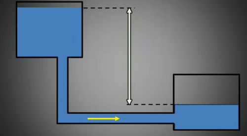
Answer: Yes. Intelligence (I), the ability to find solutions to proble-ms, is understood as the speed of the flow of electric current. In the picture on the left, the differences in the height of the liquid in two interconnected vessels give press-ure from the upper to the lower, say, voltage (V), or the potential that gives us freedom of action. There is also resistance (R) to the movement of liquid through the pipe as a kind of hierarchy for the limitations of freedom into which intelligence must fit. The formula (Voltage) = (Current)⋅(Resistance), or V = I⋅R, thus becomes similar to information perception. Without "freedom" (voltage), there is no flow, and the leakage of liquid will consume that freedom.

Abstractions are repeated in concrete phenomena, they make the subjects of perception unique, but they themselves are always incomplete (Deduction II). This is a story about mere truths, but to reach them we need vitality, an excess of freedom that dead physical matter does not have. It, the non-vital, is a foll-ower of the truth and only the truth of the reality we share, condemned to be incomplete and in turn indestructible, and yet subordinate to the intelligent. In the games of competition (Traits), the living who imitate the dead lose al-most all the games. The dead physics of nature does not descend below its surface the way the vital ones can.

Simply put, fictions are diluted information, and the vital can see it, so they can descend to their lower level of saturation with options, and sometimes even drag along with them those who cannot see such places themselves. This appeal of less information is equivalent to the greater appeal of greater proba-bility, and we use it as a "trick" to tame still life.

Hermitian IV » srb

Question: Can you explain the above to me using an easy example of a Hermi-tian operator?

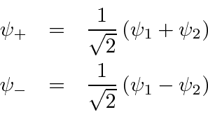
Answer: In 2-dimensional space, the Hermitian operator $\hat{T}$ (Hermi-tian III, self-adjoint $\hat{T}^\dagger = \hat{T}$) is a second-order matrix:

$$ T = \begin{pmatrix} a & b \\ b^* & c \end{pmatrix}, $$

where a, c ∈ ℝ and b ∈ ℂ. Then we have the eigenvalue equation Tv = λv, or (T - λI)v = 0, which means that the eigenvector v is perpendicular to all columns of the matrix T - λI.

1. Therefore, the determinant of this matrix is ​​zero, so:

$$ \begin{vmatrix} a - \lambda & b \\ b^* & c - \lambda \end{vmatrix} = 0, $$ $$ (a - \lambda)(c - \lambda) - b^*b = 0, $$ $$ \lambda^2 - (a + c)\lambda + ac - b^*b = 0, $$ $$ \lambda_{1,2} = \frac{a+c \pm \sqrt{(a+c)^2 - 4(ac - b^*b)}}{2}, $$ $$ \lambda_{1,2} = \frac{a+c \pm \sqrt{(a-c)^2 + 4|b|^2}}{2}. $$

It is clear that these two eigenvalues ​​are real numbers, λ_1,2 ∈ ℝ, because the expression under the root is a non-negative number, the so-called discrimi-nant of this quadratic equation D = (a - c)² + 2|b|² ≥ 0. Pauli matrices are examples of such.

2. Next, we calculate the eigenvectors v, solving (T - λI)v = 0:

$$ \begin{pmatrix} a-\lambda & b \\ b^* & c - \lambda \end{pmatrix}\begin{pmatrix} x \\ y \end{pmatrix} = 0, $$ $$ \begin{cases} (a-\lambda)x + by = 0, \\ b^*x + (c-\lambda)y = 0. \end{cases} $$

When b is a complex number, such that it is different from its conjugate (b ≠ b^*), since a - λ and c - λ are real numbers, both x and y cannot be real. This is another way of proving ((Im)Possible, 2) that Hermitian matrices with at least one complex element (now b ∈ ℂ) do not have all their eigenvectors real. Wh-en b is a real number (b = b^*), both x and y can be complex numbers, but they do not have to be.

3. To check the dependence of the above two equations, to determine that it is just one equality written in two ways, we multiply the first by b^*, and the seco-nd by a - λ, then subtract and rearrange them. We get:

[λ² - (a - c)λ + ac - |b|²]y = 0.

The expression in the brackets is identically equal to zero, which means that it is solved by more than one y. However, this multiplicity is limited by any of the two given equalities, so substitute by = (a - λ)x. Hence the corresponding eigenvectors are v_k = (b, a - λ_k)^⊤ for k ∈ {1, 2}, when we put x = b.

4. Two ways to write eigenvectors are, the second being j = {1, 2} with y = b^*:

$$ v'_k = \begin{pmatrix} b \\ a - \lambda_k \end{pmatrix}, \quad v''_j = \begin{pmatrix} c - \lambda_j \\ b^* \end{pmatrix}. $$

When we divide the vector v by the intensity, the norm of that vector ∥v∥, we get the unit vector u = v/∥v∥. To check the orthogonality of the eigenvectors, we calculate:

⟨v'₁, v'₂⟩ = v'₁^†⋅v'₂ = b^*b + (a - λ₁)(a - λ₂),
⟨v''₁, v''₂⟩ = v''₁^†⋅v''₂ = (c - λ₁)(c - λ₂) + b^*b,

4⟨v'₁, v'₂⟩ = 4|b|² + (a - c + √D)(a - c + √D),
4⟨v''₁, v''₂⟩ = (c - a + √D)(c - a - √D) + 4|b|²,

4⟨v'₁, v'₂⟩ = 4|b|² + (a - c)² - D = 0,
4⟨v''₁, v''₂⟩ = (c - a)² - D + 4|b|² =0.

Vectors v₁ and v₂ are by definition orthogonal when ⟨v₁, v₂⟩ = 0. In the link in the image above on the right you will find another proof, that the eigenvectors of Hermitian operators are mutually orthogonal. When we divide these vecto-rs by their intensities we obtain a system of orthonormal vectors.

5. Theorem. Given n ∈ ℕ different eigenvalues ​​λ ∈ ℝ and the same number of orthonormal vectors v, an (unknown) Hermitian matrix can be formed, with an auxiliary matrix P columns of the given vectors v and D diagonal matrix of the given eigenvalues ​​λ, of the form T = PDP^†.

Proof: The matrix T is Hermitian, because:

T^† = (PDP^†)^† = (P^†)^†D^†P^† = PDP^† = T.

Then, Tv = (PDP^†)v = (PD)P^†v, and I_k = P^†v is a matrix that has 1 in the k-th row of the k-th column and all other zeros, if v is a vector in its k-th row. Then (PDP^†)I_k = P(DI_k) = PD_k, where λ_k is in the k-th row of the k-th column, while the other elements of that matrix are zero. Finally, PD_k = λ_kv_k and that v_k is the starting v that was k-th in its sequence, i.e. Tv = λv. Therefore, we have the eigenvalues ​​λ of the eigenvectors v of the matrix T. ∎

But this is a rich and special topic.

Unitary II » srb

Question: What are unitary operators?

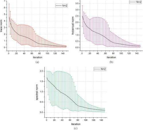
Answer: A unitary operator is a linear transformation of a Hilbert space (complete vector space, with a scalar product, which generalizes to the Euclidean space) that preserves scalar products and norms, me-aning that it does not change the length or angle between vectors. It is an invertible operator where its adjoint is equal to its inverse U^† = U^-1. This property is fundamental in quantum mechanics for describ-ing the time evolution of quantum systems while preserving probabilities (Unitary).

In the previous theorem (Hermitian IV, 5) the auxiliary matrix P is unitary. The image link on the left is an article from quantum computing, as an exam-ple in which quantum machine learning is described using unitary operators. Every dimensionless Hermitian operator  will give exp(iÂ) a unitary operator, so exp(iΔtH/ℏ) is unitary when H is Hamiltonian. Then the unitary ope-rator exp(ipΔx/ℏ) translates the ket state by -Δx. Conversely, the unitary op-erator exp(ixΔp/ℏ), it translates the ket state by Δp in momentum space. The unitary operator exp(iL_zΔθ/ℏ) rotates the ket state by an angle -θ. These are just some easy and well-known examples of the application of unitary operators.

Manipulation of a quantum system maps to working with the appropriate unitary matrices. When we have a Hamiltonian, a Hermitian operator $\hat{H}$ that represents the total energy of a given system, we use it to work with the unitary operator:

$$ \hat{U} = e^{-\frac{i}{\hbar}\hat{H}t} $$

during time t, where ℏ = h/2π. Given the precision of that simulation, with a small allowed error ε > 0, a quantum interpretation for the operator Û is sought that approximates the target unitary operator Û₀ such that:

|Û - Û₀| ≤ ε.

This is also the task of searching for quantum algorithms (quantum circuits) of the aforementioned machine learning.

1.Due to the assumed property of preserving the length of a vector in a mapping:

∥Ûv∥² = ⟨Ûv, Ûv⟩ = ⟨v, Û^†Ûv⟩ = ⟨v, v⟩ = ∥v∥²

Unitary operators have interpretations in the conservation laws of physics. They therefore copy observables into analogous observables, that is, in vector terms, the unitary operator Û will copy every orthonormal basis from the space X into some orthonormal basis of that same X.

Namely, let ⟨u_j, u_k⟩ = δ_j,k for the set of orthonormal vectors u₁, u₂, ... ∈ X of the given vector space. Then, by the definition of the unitary operator ⟨Ûu_j, Ûu_k⟩ = ⟨u_j, u_k⟩, which means that the new set of vectors w_k = Ûu_k is also orthonormal, i.e. ⟨w_j, w_k⟩ = δ_j,k. The Kronecker delta is δ_j,k = 0 when j ≠ k, but is δ_j,k = 1 when j = k.

2. If one orthonormal basis {u₁, u₂, ..., u_n} is transformed into another {v₁, v₂, ..., v_n} by the unitary operator Û : u → v, then the matrix of this operator will be the same in both bases. This is a special case of the more general theorem that states that an operator that transforms one set of basis vectors into another has the same matrix elements in both bases. However, in the case of unitary operators, the proof is particularly simple:

Û_jk{u} = ⟨u_j, Ûu_k⟩ = ⟨u_j, v_k⟩ = ⟨Û^-1v_j, v_k⟩ =
= ⟨Û^†v_j, v_k⟩ = ⟨v_j, Ûv_k⟩ = Û_jk{v}.

This particularly facilitates working with unitary matrices, representing unitary operators in given bases.

3. The characteristic equation Uv = λv, say of the unitary matrix U, its eigen-value λ and the associated eigenvector v, by adjunction (conjugation and transposition) will give v^†U^† = v^†λ^*. We also write it like this:

U|v⟩ → ⟨v|U^† = ⟨v|λ^*.

We combine the multiplications and find:

∥v∥² = ⟨v|v⟩ = ⟨v|U^†U|v⟩ = ⟨v|λ^*λ|v⟩ = λ^*λ⟨v|v⟩ = |λ|²∥v∥²,

so if ∥v∥ ≠ 0, then |λ|² = 1. Thus, the eigenvalues ​​λ of a unitary matrix are unimodular, that is, they have norm 1; they can be written as e^iα for some α.

4. This leads to another important property. As in the case of Hermitian matrices, the eigenvectors v_k of unitary matrices, corresponding to different λ_k = e^iα_k eigenvalues, are orthogonal. Namely:

U|v_j⟩ = e^iα_j|v_j⟩,     U|v_k⟩ = e^iα_k|v_k⟩,

⟨v_j|e^iα_j|v_k⟩ = ⟨v_j|U|v_k⟩ = ⟨v_j|e^iα_k|v_k⟩,

(e^iα_j - e^iα_k)⟨v_j|v_k⟩ = 0,

so if e^iα_j ≠ e^iα_k, then ⟨v_j|v_k⟩ = 0. Therefore, the above theorem (Hermitian IV, 5) also holds for unitary matrices.

5. Finally, here are some examples of unitary matrices:

$$ U_1 = \frac{1}{\sqrt{2}}\begin{pmatrix} 1 & i \\ i & 1 \end{pmatrix}, \quad U_2 = \begin{pmatrix} e^{i\alpha} & 0 \\ 0 & e^{i\beta} \end{pmatrix}, $$ $$ U_3 = \begin{pmatrix} i & 0 & 0 \\ 0 & i & 0 \\ 0 & 0 & i \end{pmatrix}. $$

Unitarity is checked by multiplying the conjugate transpose by the given matrix, if the result is a identity matrix, U^†U = I. We design them as needed to correspond to some phenomenon for which the conservation law holds, and then analyze these mathematical forms instead of experimenting with the phenomena themselves. This is not just about saving money, but also about (mathematical) precision.

Simulations IV » srb

Question: Why do you recommend unitary operators in simulations?

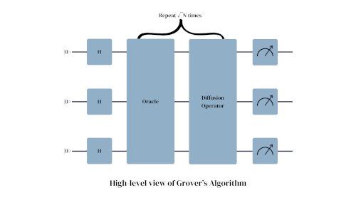
Answer: I do simulations as a hobby, to test an idea, or to check on a question you send me. Now I do it mostly sporadically and unsystematically, but it used to be my profession also.

As you can see in the link on the right, it is common practice today that every operation implemented in a quantum computer must follow a unitary matrix. Also, note that the author of the text talks about Grover's Аlgorithm for searching random data as if it were some kind of game and competition. Note that taming nature is also kind of competitive game. Unitary operators are the basis of game simulation within quantum game theory, representing player strategies and governing the evolution of the system.

I am particularly interested in a detail about dual perception that may not be widely noticed (Conjugated). The world we see is dual to what it is, but not in some superficial sense but in a deeper way, which we can connect with the duality of space metrics (Lp spaces). This has been a topic here many times (Dualism II), but not in the following way. Before that, we should note the difference between co- and contra-variant vectors (Variance). The former are coordinates that follow the coordinate axes, and the latter are orthogonal projections onto those axes, and the difference arises when we leave Cartesian rectangular coordinates.

The scalar product in this sense of dual vectors is invariant, otherwise it is not (Invariant II). This gains importance in Information Perception which, by the scalar product of vectors, i.e. the states of subjects, expresses the possibility of their mutual interactions (perceptions). Like many other types of information, this coupling is also subject to the law of conservation and exists as reality, and is condemned to isometries and then to unitary operators. Here we come to the question posed to us.

For example, the volume of memory (after the Big Bang) will grow with the cube of the radius (ball $V = \frac43r^3\pi$), but the surface (sphere $S = 4r^2\pi$) only with the square of the radius (r), so the ability to radiate the present to the past decreases with the radius (S/V = 1/3r), we can say with the duration (t = r/c). However, the units of duration and units of length change, relatively to the saturation with information. Since the current present has less and less uncertainty, its time flows more slowly (there are fewer events), so the relative time of the past seems faster to us. The units of space are getting longer radially (from us) and as such we see wavelengths of light from ever more distant galaxies. I mention this "speculation" only as a curiosity, actually irrelevant to the explanation that follows.

In a possible communication U between a subject and an object, vectors or states x and y, when we calculate the perceptual information S = ⟨x|y⟩, what the object sends is U|y⟩ and what the subject receives is ⟨x|U^†. The result, the scalar product or perceptual information is an invariant:

⟨x|U^†U|y⟩ = ⟨x|I|y⟩ = ⟨x|y⟩ = S.

Now written using unitary operators, or matrices of such, this is what perceptual information is anyway.

Example. Let's show on the unitary matrix (U₁) from the previous example:

$$ U = \frac{1}{\sqrt{2}}\begin{pmatrix} 1 & i \\ i & 1 \end{pmatrix} $$

the importance of the aforementioned dual multiplication.

Solution: Matrix multiplications give:

$$ UU = \frac{1}{\sqrt{2}}\begin{pmatrix} 1 & i \\ i & 1 \end{pmatrix} \frac{1}{\sqrt{2}}\begin{pmatrix} 1 & i \\ i & 1 \end{pmatrix} = \frac12\begin{pmatrix} 0 & 2i \\ 2i & 0 \end{pmatrix} = \begin{pmatrix} 0 & 1 \\ 1 & 0 \end{pmatrix}, $$ $$ U^\dagger U = \frac{1}{\sqrt{2}}\begin{pmatrix} 1 & -i \\ -i & 1 \end{pmatrix} \frac{1}{\sqrt{2}}\begin{pmatrix} 1 & i \\ i & 1 \end{pmatrix} = \frac12\begin{pmatrix} 2 & 0 \\ 0 & 2 \end{pmatrix} = \begin{pmatrix} 1 & 0 \\ 0 & 1 \end{pmatrix}. $$

Therefore, incorrect and correct scalar multiplications would give:

$$ \langle x|UU|y\rangle = \begin{pmatrix} x_1 & x_2 \rangle \end{pmatrix} | \begin{pmatrix} 0 & 1 \\ 1 & 0 \end{pmatrix} | \begin{pmatrix} y_1 \\ y_2 \end{pmatrix} = x_2y_1 + x_1y_2, $$ $$ \langle x|U^\dagger U|y\rangle = \begin{pmatrix} x_1 & x_2 \rangle \end{pmatrix} | \begin{pmatrix} 1 & 0 \\ 0 & 1 \end{pmatrix} | \begin{pmatrix} y_1 \\ y_2 \end{pmatrix} = x_1y_1 + x_2y_2. $$

Direct multiplication is wrong, dual is correct. ∎

January 2026 (Original ≽)