November 2026 (Original ≽)

Isometry III » srb

Question: What is the difference between isometry and symmetry?

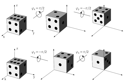
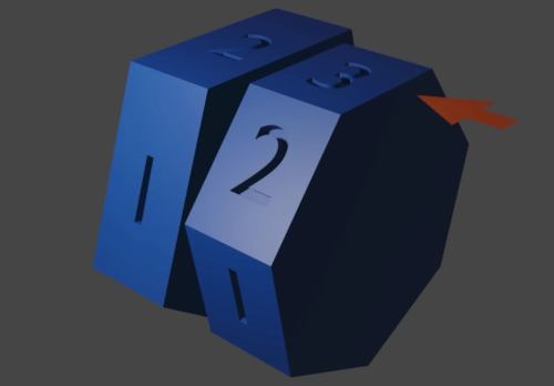
Answer: Isometry is a transformat-ion of space that preserves the gro-wths between points, while symme-try is an invariant property, where a given physical law, phenomenon, or object remains unchanged while the rest is transformed. Within ma-thematics, isometry is also called congruence. They are: reflections (central, axial, mirror symmetry), translations, rotations. They can all be reduced to only rotations. Succe-ssive rotations (in the image with a dice) may be non-commutative. In curved spaces (gravity) translation may change the direction of the vector.

1. We know that on a flat, Euclidean surface, the Pythagorean theorem holds for right triangles: the sum of the squares of the legs is equal to the square of the hypotenuse. This also holds for infinitesimal triangles, so:

ds² = dx² + dy²,

where the infinitesimal lengths dx and dy are the legs starting from the origin of the rectangular coordinate system (OXY), and ds is the hypotenuse. When we move the points of the triangle by a constant vector (a, b), we get d(x + a) = dx + da = dx and d(y + b) = dy, because the differentials of constants are zero. This is a translation as an example of isometry, because the length of the hyp-otenuse ds remains unchanged.

2. Another example, coordinate transformation:

$$ u = a_{11}x + a_{12}y, \quad v = a_{21}x + a_{22}y. $$

According to the rules of differentiation, we find:

$$ \begin{cases} dx = \frac{\partial x(u,v)}{\partial u}du + \frac{\partial x(u,v)}{\partial v}dv = a_{11}du + a_{12}dv \\ dy = \frac{\partial y(u,v)}{\partial u}du + \frac{\partial y(u,v)}{\partial v}dv = a_{21}du + a_{22}dv \end{cases} $$

or matrix:

$$ \begin{pmatrix} dx \\ dy \end{pmatrix} = \begin{pmatrix} a_{11} & a_{12} \\ a_{21} & a_{22} \end{pmatrix} \begin{pmatrix} du \\ dv \end{pmatrix}, $$ $$ d\vec{z} = Jd\vec{w}. $$

These results are also valid when the coefficients a_ij ∈ ℝ are not constants but do not depend on the coordinates x, y ∈ ℝ. The matrix J is called the Jacobian, and its determinant |J| expresses the area (n-volume, n-dim space) part which it refers, so that the corresponding new area dx dy = |J| du dv. This maintains the invariant, the immutability of the surface (volume if the space is 3-dimens-ional) element of the space of transformed coordinates.

3. When points (x, y) have additional values, say, densities expressed by the function f(x, y), parts of the surface will remain of the same mass when:

f(x, y)dx dy = g(u, v) |J| du dv,

where the density is the same, in the new variables, g(u, v) = f(x(u, v), y(u, v)), then stretched or contracted depending on the stretching or contracting of the parts of space by the transformation. It is also a type of invariant (of total ma-ss, force field strength, heat, and the like).

However, the Pythagorean theorem takes the form:

ds² = dx² + dy² = (a₁₁du + a₁₂dv)² + (a₂₁du + a₂₂dv)²,

ds² = (a₁₁² + a₂₁²)du² + 2(a₁₁a₁₂ + a₂₁a₂₂)dudv + (a₁₂² + a₂₂²)dv²,

ds² = g₁₁du² + g₁₂dudv + g₂₁dvdu + g₂₂dv².

The coefficients g_ij are elements of a metric tensor, doubly covariant (due to the two subscripts). The expression written with them is the same value of the hypotenuse in the new coordinates. It is also an invariant, now of length. If the coordinates (u, v) are orthogonal, for i ≠ j then g_ij = 0, the mixed coefficients of the metric tensor are always zero.

4. As we can see, isometry emphasizes the same measurability that in symmet-ry is invariance in general, and otherwise they are quite related areas. The co-ncept of variability is always applicable in the finite world of our perceptions, or physical interactions, and so is the concept of measurability. The same can be said for countable infinity, say the set of natural numbers ℕ, but uncounta-ble infinity, for example (Vitali) of real numbers ℝ, also has immeasurable se-ts. According to the current scope of quantum mechanics, I am of the opinion that such immeasurable sets exist in superpositions.

Manifold II » srb

Question: How do mathematicians view space?

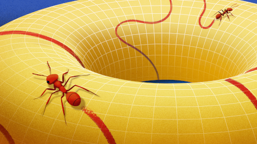
Answer: A manifold is such an abs-tract topological space in which ea-ch point has a neighborhood with the properties of Euclidean space, but may be part of a complex larger structure.

For example, a circle is a one-dim-ensional manifold. Zoom in anyw-here on it and it will be a straight line. An ant living on a larger circle will not know that the path is actually circular. But zoom in on a figure eight, right at the point where it intersects itself, and it will never look like a straight line. An ant would realize at that intersection that it is not in Euclidean space. The figure eight is therefore not a manifold.

Riemann (1854) presented the concept of manifolds, curves and surfaces ind-ependent of the space surrounding them, in a lecture in Göttingen, extending Gauss's ideas of geometry to arbitrary dimensions, even infinite ones, but it was not understood until two years after his death (1868). By the end of the 19th century, mathematical giants such as Henri Poincaré still recognized Ri-emann's ideas, and in 1915 Albert Einstein used them in his general theory of relativity.

1. In mathematics, a Lie group is also a smooth manifold, where the group op-erations are smooth functions of the elements of the group. Lie groups are im-portant in mathematical analysis, physics, and geometry because they express symmetries of various structures. The concept of a group is the essence of sy-mmetry, and we recall that a group (G,∗) is the set G of the binary operations ∗ and the axioms (∀a, b, c ∈ G):

• Closure: a∗b ∈ G;
• Associativity: (a*b)*c = a*(b*c);
• Neutral: (∃e ∈ G)(∀a ∈ G) e*a = a*e = a;
• Inverse: (∀a ∈ G)(∃b ∈ G) a*b = b*a = e.

It can be shown that the inverse b of a given element a is unique, and that the left and right inverses of an element are the same. A group G is Abelian or commutative if the operation is commutative, that is, for each a, b in G, a∗b = b∗a. A commutative discrete group is (ℤ, +) with neutral element 0 and for each integer z ∈ {0, 1, -1, 2, -2, ...} the inverse -z. A general linear Lie group of degree 2 consists of regular second-order matrices:

$$ \text{GL}(2) = \{ A = \begin{pmatrix} a & b \\ c & d \end{pmatrix}: \det A \ne 0 \}. $$

When the coefficients of these matrices are real numbers (a, b, c, d ∈ ℝ), it is a 4-dim noncompact real Lie group, a subset of ℝ⁴. We call it disconnected bec-ause it has two connected components containing these matrices with positive and negative determinants. Its subgroup, denoted SO(2), is the rotation matr-ices of unit determinant. The space-time isometries of the theory of relativity (Minkowski) are also Lie groups. The Heisenberg group (H3) of quantum me-chanics is also a Lie group, and so on.

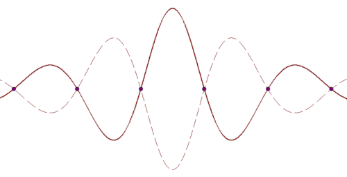
2. We know that by measuring a pa-rticle-wave, the particle itself and its former trajectory are formed (Heisenberg, 1927). At the same ti-me the amplitudes of the resulting waves, in the figure on the left, de-fine the probability of finding the particle in the measurement (in terms of the squares of the modu-lus). These probabilities are zero at the nodes, which makes these positions appear discrete (atomized). As the co-llapse of the superposition into a particle-wave results in its quantization, it passes from the continuum of the lower world to the discrete upper world of physical reality. In this way, I understand the continuity of the space of Sch-rödinger's differential equation and the discontinuity in the periodicity of the obtained solutions, wave functions ψ. Therefore, the space of quantum supe-rpositions is a manifold, unlike the positions of quantum particles.

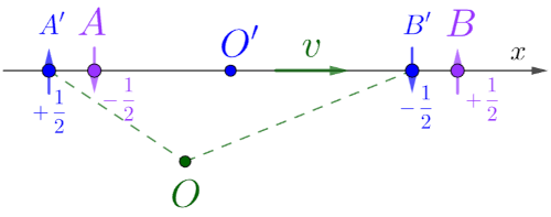
3. The image on the right shows qu-antum entanglement. Here A' and B' are simultaneous events for O' and non-simultaneous for O, resu-lting from the decay of some parti-cle. Their spins ±1/2 sum to zero, although at no time can it be known which is + and which is -. This is a system moving with a velocity v on the abscissa relative to O and Anna (A) and Boban (B) would measure the spin of these events at (almost) the same time.

Even when v = 0, the pairs of distances of the events from any observers of the abscissa, except O', are not the same and these events are not simultaneous to them. However, the distances of A and B from O' can be planned to be the sa-me and, as we know, say, when Anna measures spin -1/2 Boban measures spin +1/2. This is a well-known quantum entanglement and now let's add somethi-ng like the previous observation (2). As the events A' and B' move away, their present (simultaneity) will go into the more recent future and, for Anna and Boban, will be like a probability wave (2). Namely, it also has zero probability nodes, places and moments when it is there and then it is not. We calculate it as manifolds that are projected into the discreteness of the observer's reality.

4. The source O' that is moving, v > 0, in addition to different energy and mo-mentum, has shortened units of length and a slowed-down time flow relative to the observer from O and sees the particle-waves A' and B' differently than from the source that is at rest. And the changes in the measures of path and duration reveal to us that the space-time that they can build is, or is approx-imately so given the discreteness of physical observations, a continuum. In this sense, the possibilities from which these particle-waves come are mani-fold.

Another way we find it is by counting. For example, the flickers of photons and vacuum, or any other particle, or phenomenon or process that would flow ind-efinitely through the universe, are discrete. These are countable sequences of reality with an infinite subsequence of possibilities and whose cardinality is a continuum. As in the case of digits (decimal or binary) from 0 to 1. In order to have multiplicity, we need this smoothness of the continuum, and we have it in mathematics and, therefore, it is somewhere next to us.

Modulo » srb

Question: Can you explain modular arithmetic to me?

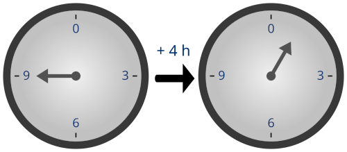
Answer: Modular arithmetic is the return of numbers to a circle inven-ted by Gauss (1801), as in the clock in the picture on the left, where:

(9 + 4) (mod 12) = 1.

Moduo (or modulo) is a remainder operation that returns the remaind-er of the quotient of two integers. It is often denoted by the mod sign or the percentage (%) in programming. Given two numbers, a (divisor) and n (divid-er), we write:

a (mod n) = r

where r is the remainder for which 0 ≤ r < n. For example, 23 (mod 5) = 3, be-cause 23 = 4⋅5 + 3. In general, a = n⋅m + r.

1. Let us show that the rule of addition of modules (a, b, n ∈ ℕ) holds:

(a + b) (mod n) = [a (mod n) + b (mod n)] (mod n).

For example, (14 + 0) (mod 5) = [14 (mod 5) + 9 (mod 5)] (mod 5) =

[4 + 4] (mod 5) = 8 (mod 5) = 3,

which is correct.

In general, from (a + b) (mod n), it follows:

a + b = m⋅n + r,
a + b = (m_a + m_b)⋅n + r_a + r_b,
a + b = (m_a⋅n + r_a) + (m_b⋅n + r_b),

where m_a + m_b = m and r_a + r_b = r, which proves the statement.

2. To make this easier to apply to subtraction, we write:

a ≡ b (mod n)

and this we read “a is congruent to b modulo n” with the meaning that given natural numbers a and b have equal remainders after division by the natural number n. For example, 13 ≡ 23 (mod 5), so when we apply rule (1) to negative numbers and add -15 to both sides, we find -2 ≡ 8 (mod 5). A little more clear-ly, it will be -2 ≡ 3 (mod 5), so that the sum of the negative and positive diviso-rs (a + b) is divisible by the divider (n). Hence the subtraction (a, b, n ∈ ℕ):

(a - b) (mod n) = [a (mod n) - b (mod n) + n] (mod n),

where we add the divider n in square brackets, possibly multiple times, to avo-id negative numbers for the moduli. For example:

(17 - 39) (mod 5) = [17 (mod 5) - 39 (mod 5) + 40] (mod 5),
-22 (mod 5) = [2 + 1] (mod 5),
(25 - 22) (mod 5) = 3 (mod 5),
3 (mod 5) = 3 (mod 5),

and that is the number 3, i.e. -22 ≡ 3 (mod 5).

3. Let us show that for multiplication:

a⋅b (mod n) = [(a (mod n))⋅(b (mod n))] (mod n).

For example:

7⋅4 (mod 5) = [(7 (mod 5))⋅(4 (mod 5))] (mod 5),
28 (mod 5) = [(2)⋅(4)] (mod 5),
(5⋅5 + 3) (mod 5) = (5 + 3) (mod 5),
3 = 3,

and this is a true equality. In general (all numbers are natural):

a = m_an + r_a,     b = m_bn + r_b,

a⋅b = (m_an + r_a)⋅(m_bn + r_b) =
= (m_am_bn + m_ar_b + m_br_a)n + r_ar_b,

a⋅b = mn + r.

The above formula follows from this pattern.

For example, 123⋅456 (mod 5) = 3⋅6 (mod 5) = 3. Indeed, 123⋅456 = 56088, which is a number with a remainder of 3.

4. From this, the formula for the modulus of the degree follows directly:

a^k (mod n) = [a (mod n)]^k (mod n).

For example:

123¹⁰ (mod 5) = 3¹⁰ (mod 5) = 3⁴⋅3⁴⋅3 (mod 5) =
= 81⋅81⋅3 (mod 5) = 1⋅1⋅3 (mod 5) = 1⋅1⋅3,

123¹⁰ (mod 5) = 3.

The usual division, a:b (mod n), does not exist in modular arithmetic.

5. Modular arithmetic is a well-known and oversimplified topic for this theory, but I have included it because of Alan Turing's (1936) halting problem, which revealed a contradiction in the idea that there is an algorithm that would deci-de whether a computer program, or any algorithm for a given task, will finish its work or continue to execute indefinitely. It is also the problem of the liar paradox (Three-valued, 3) which says: "I am lying.", from which I see the so-lution that the subject, or the decision-making system in general, cannot judge itself well. For example, mathematics' proof of its own correctness is invalid, and therefore Gödel's impossibility theorems establish that mathematics can-not prove its own truth. In the case of modular arithmetic, this is the inability of a "counting system" to determine from within, without external help, whet-her it is going in a circle. Just as a consistent system, of truths and only truths, is not complete, i.e. there is always some truth that it cannot prove, and by co-mbining lies (incorrect ⊥ with correct ⊤ statements) mathematicians can brid-ge these islands of truth.

Disease » srb

Question: Did I understand correctly that you are saying a closed system, wh-en making decisions about itself, resembles a patient who cannot be cured wi-thout external help or additional intervention from doctors?

Answer: An interesting observation and a good metaphor. This is the discovery of Turing's halting parad-ox. Assuming that there is an inte-rnal monitoring system that would recognize the blockage of the syst-em of processes in which it is in order to prevent the system from entering that state, it would find itself in a state before entry when it could not recognize the blockage and would enter the system and be blocked. This is the contradiction of the "Halting Problem". It tells us that ne-ither a computer nor any algorithm can (always) be its own doctor, originally an evaluator.

1. This is the weakness of a closed system that is overcome by separating indi-viduals as separate entities, by their freedom, either with the principle of mini-malism (of living beings) or its narrower part: the principle of least action (of physics). Also by tracing the evolution of life, by random discovery, because more than 99% of all species that have ever lived on Earth during its 3.5 bill-ion-year history have become extinct. Hence, the success of life on Earth is also a consequence of its diversity as a counterpoint to the described blocka-ges, the failures of closed systems.

2. This distancing in order to form a separateness is not a feature of life alone, nor does it arise only because of the "halting difficulty", but also comes from a principled minimalism and a departure from a homogeneous distribution that has too much uncertainty, but also with all the third possible reasons that are not known to us for now, or never will be, but which are consequences of the correctness of mathematics and its breadth. Consequently, there are the cau-ses of the collapse of empires (Crumble) to, at the other extreme, the disinte-gration of particles. The superposition will collapse from a state of ambiguity into a single meaning, like the outcome of a coin toss, entering a state of im-possibility of its own evaluation, let's say (metaphorically) making wrong de-cisions, when it risks falling behind with its new and current reality from the rest of the present, which is otherwise moving at the speed of light into the future, into a new physical reality.

3. The same distancing and emergence of singularity, is similar to vitality in terms of excess freedom for questions of the principle of least action of physi-cs. Then, singularity shortens its own duration in relation to reality, and thus also truthfulness in the sense of my theory (a greater truth requires a greater minimum number of steps to contradiction). Particle-waves flicker because they are information structures, and every piece of news communicated ceases to be news, but are now attempts at fictions and their realizations in particles. Also, we observe the mathematical basis of the cosmos in the construction of the world of physics where mathematics as a complete truth cannot speak about itself and is expressed through materiality, which again its representa-tion can inspire but not prove mathematics.

4. There are many such metaphors about an incurable disease of a patient wi-thout outside help, and their essence is the impossibility of making a correct (mathematical, yes-no) decision within a given system on some issues of the system itself. We know some examples of indecision well. We experience me-nu overload when we stand in front of a restaurant menu for a long time, read-ing numerous options, only to end up giving up on the order in frustration. A similar example is the “perfectionist’s dilemma” who believes that there is one “perfect” choice and that making a mistake is unacceptable to him, so he rem-ains indecisive. In mathematics, these are, for example, problems without so-lutions, such as polynomials of the fifth degree and higher that cannot be solv-ed by squaring, or an irrational number that cannot be written as the quotient of two integers. I will skip the less trivial cases, because the point of the ques-tion has been achieved: there is no success without breakthroughs.

Lagrangian III » srb

Question: Do you have any examples of using the Euler-Lagrange equation?

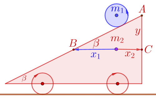
Answer: First look at the easier ex-amples of spring and gravity, in the book Space-Time (1.2.8-9.), then Theorem 1.2.10. which establishes that the Euler-Lagrange formula:

$$ \frac{d}{dt}\left( \frac{\partial L}{\partial \dot{x}_0}\right) = \frac{dL}{dx_0}, $$

with the Lagrangian L = E_k - E_p, i.e. kinetic minus potential energy, of all functions x(t) of fixed ends, calculates the stationary trajectory x₀(t), local minimum, maximum or slope. See an introductory example (Block on a Slo-pe), and I will explain this in the picture, also school, example of using the Euler-Lagrange equation.

1. A globe of mass m₁ rolls down a steep incline β, traveling from A to point B, the projections of which are on the abscissa x₁ and on the ordinate y. This slo-pe is part of a cart of mass m₂, which, due to the reaction, rolls away by x₂ in the opposite direction. Let's ignore friction and find the acceleration of the cart.

In short, the vertical acceleration of gravity of the globe decreases with the tangent of the angle beta, and its momentum to the left has a reaction mom-entum of the cart to the right. This is a process that we will now express more precisely.

2. The tangent of the angle β is the ratio of the opposite y and the adjacent x₁+x₂ leg of the right triangle ABC, hence y = (x₁+x₂)⋅tg β. This Lagrangian is L = E_k - E_p. The kinetic energy E_k = E_k1 + E_k2 of this system has two parts, the globe and the cart, respectively:

$$ E_{k1} = \frac12m_1 [\dot{x}_1^2 + (\dot{x}_1 + \dot{x}_2)^2 \tan^2 \beta], \quad E_{k2} = \frac12m_2 \dot{x}_2^2, $$ $$ E_k = \frac12 (m_1\dot{x}_1^2 + m_2\dot{x}_2^2) + \frac12 m_1 (\dot{x}_1 + \dot{x}_2)^2 \tan^2 \beta. $$

The potential energy E_p = E_p1 + E_p2 has the sums:

$$ E_{p1} = -m_1g\, (x_1 + x_2)\tan\beta, \quad E_{p2} = 0, $$

so the Lagrangian is:

$$ L = \frac12 (m_1\dot{x}_1^2 + m_2\dot{x}_2^2) + \frac12 m_1 (\dot{x}_1 + \dot{x}_2)^2 \tan^2 \beta + m_1g\,(x_1 + x_2)\tan\beta. $$

The derivative of distance with respect to time, i.e. ẋ, is the velocity, and $g = \ddot{x}$ is the gravitational acceleration (the derivative of velocity with respect to time).

3. The derivatives of the Lagrangian along the paths are equal to:

$$ \frac{\partial L}{\partial x_1} = \frac{\partial L}{\partial x_2} = m_1g\,\tan \beta . $$

However, the speed derivatives are:

$$ \frac{\partial L}{\partial \dot{x}_1} = m_1\dot{x}_1 + m_1(\dot{x}_1 + \dot{x}_1)\tan^2 \beta, \quad \frac{\partial L}{\partial \dot{x}_2} = m_2\dot{x}_2 + m_1(\dot{x}_1 + \dot{x}_2)\tan^2 \beta, $$

and their derivatives with respect to time:

$$ \frac{d}{dt}\frac{\partial L}{\partial \dot{x}_1} = m_1\ddot{x}_1 + m_1(\ddot{x}_1 + \ddot{x}_2)\tan^2\beta, , \quad \frac{d}{dt}\frac{\partial L}{\partial \dot{x}_2} = m_2\ddot{x}_2 + m_1(\ddot{x}_1 + \ddot{x}_2)\tan^2\beta. $$

We have obtained (two each) sides of the two Euler-Lagrange equations.

4. We found two Euler-Lagrange equations, the motion of the globe and the cart:

$$ \begin{cases} m_1\ddot{x}_1 + m_1(\ddot{x}_1 + \ddot{x}_2)\,\tan^2\beta = m_1g\, \tan \beta, \\ m_2\ddot{x}_2 + m_1(\ddot{x}_1 + \ddot{x}_2)\,\tan^2\beta = m_1g\, \tan \beta. \end{cases} $$

We write them as linear acceleration systems:

$$ \begin{cases} m_1(1 + \tan^2\beta)\ddot{x}_1 + (m_1\, \tan^2\beta)\ddot{x}_2 = m_1g\, \tan \beta, \\ (m_1\, \tan^2\beta)\ddot{x}_1 + (m_2 + m_1\, \tan^2 \beta) \ddot{x}_2 = m_1g\, \tan \beta. \end{cases} $$

One of the two solutions to this system is to accelerate the cart:

$$ \ddot{x}_2 = \frac{m_1g \sin\beta \cos\beta}{m_2 + m_1\sin^2\beta}. $$

That is the desired result of the given task.

5. The next example is also about the use of the Euler-Lagrange equation. It has two parts. The first comes with the universality and stationarity of these equations themselves. This reveals to us the constant balances of physical re-ality, from the surface of calm water to the largest storms. A constantly bala-nced reality is always correct, true. When we really prove that something can-not happen, it will not happen in an experiment. This is the second part from which it emerges that abandoning the E-L solution means a step into the un-real, I say fictitious, into half-truths and untruths. On that side is a “living” being, which I define as a system that can lie at will. It will have some “intel-ligence” in the sense of the ability to bring given tasks, states or processes into information that would not be normal, current, or natural states for it.

Free will arises through the union (emergence) of dead physical matter and "vitality", and with its help we defy the principle of least action in physics. Inf-ormation has various definitions, always as quantities of uncertainty. But in this form it is a good basis for drawing the boundaries of the solutions of the E-L equations, that is, these equations help to recognize the scope of inform-ation. That is the deeper meaning of this last "example".

Evenness » srb

Question: What connects Newtonian, Lagrangean, and Hamiltonian mechani-cs?

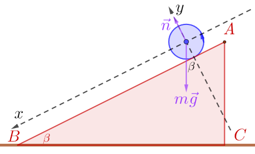
Answer: Typically, for school exa-mples of solutions to motion using forces, Lagrangians and Hamiltoni-ans, a steep plane is used. The figu-re on the right shows an example of rolling (frictionless) a ball of mass m along the side AB of an inclinati-on β. Unlike the upper inclined pl-ane, this one is stationary. This ball is again pulled by the gravitational force $m\vec{g}$ towards the base (BC),but the abscissa is placed parallel to the slope, in the direction of rolling through the center of the ball in its initial position when it is at rest, through which the ordinate also passes perpendicular to it.

Thus, the picture is suitable for the application of Newton's method. We consi-der it, also Lagrange's and Hamilton's to make sure that all three give the sa-me equations of motion. It turns out that these are three equivalent methods (for describing motion), and I consider the mapping of solutions through the-se three ways of searching to be another (unrecognized) type of symmetry of these methods themselves.

1. Newton's force is the product of mass and acceleration $\vec{F} = m\vec{a}$. In general, acceleration ($|\vec{a}| = \ddot{s} = \frac{d\dot{s}}{dt}$) is known as the change in velocity ($\dot{s} = \frac{ds}{dt}$) over time ($t$), and velocity is the change in distance ($s$) over time. In this sketch, the ground force ($\vec{n}$) is normal, perpendicular to the abscissa, and there is no acc-eleration due to the ball rolling $\ddot{y} = 0$, so $\vec{n} = 0$. The total gravitational force $mg = m|\vec{g}|$ is projected onto the slope of the angle β and reduced:

$$ \ddot{x} = g \sin \beta. $$

Otherwise, we obtain the velocity $\dot{x} = g\sin \beta + \dot{x}_1$ by integrating the accelera-tion. Now there is no initial velocity, $\dot{x}_1 = 0$. The path:

$$ x = \frac12 g \sin \beta t^2 + \dot{x}_1 t + x_0 $$

is the integral of the velocity, where the initial position is again zero, $x_0 = 0$, the origin of the system.

2. The Lagrangian, L = E_k - E_p, is the difference of kinetic, $E_k = \frac12 m \dot{s}^2$, and potential, $E_p = -mgs\sin\beta$, energies, where s is the distance the ball travels along the slope. The former is the semi-product of the ball's mass m and the square of its velocity $\dot{s}^2 = \dot{x}^2 + \dot{y}^2$, and the latter is the product of the mass, the gravitational acceleration, and the height h = s⋅sin β projected onto the slope. Now the abscissa (x-axis) is the line of the base, the ordinate (y-axis) goes perpendicular to the abscissa and through the center of the globe at the initial moment ($t = 0$, $\dot{s} = 0$). Hence the Lagrangian:

$$ L = \frac12m(\dot{x}^2 + \dot{y}^2) + mgh, $$ $$ L = \frac12 m \dot{s}^2 + mgs\sin\beta. $$

In this case, the gravitational potential can also be calculated with E_p = mgy, where y = mg(y₀ - h), with the initial height of the ball y₀ and h = s⋅sin β the actual height of the fall, but the result will be the same because y₀ is a const-ant.

Then we calculate the derivatives of the Lagrangian, substitute, and subtract the mass:

$$ \frac{dL}{ds} = mg\sin\beta, \quad \frac{\partial L}{\partial \dot{s}} = m\dot{s}, \quad \frac{d}{dt}\frac{\partial L}{\partial \dot{s}} = m\ddot{s}, $$ $$ \ddot{s} = g\sin\beta. $$

By integrating the acceleration over time we obtain the velocity, and by inte-grating the velocity we find the distance traveled. These results are equal to Newton's (1).

3. The transition from preserving the stationarity of Lagrangian (L = T - V), the difference between kinetic and potential energy, to preserving their sum, i.e. the Hamiltonian (H = T + V), has already been stated in general form (No-ether, 4), and now let's look at it using the example of an inclined plane. The relationship between the Hamiltonian and the Lagrangian is often written with generalized coordinates of the momentum and position of individual particles, p_j and q_j, a set of variables that fully describe the position, arrangement, and state of a physical system at any given moment:

$$ H = \sum_{j=1}^n p_j\dot{q}_j - L, \quad p_j = m\dot{q}_j, \quad j = 1, 2, ..., n, $$

where now we have only one "particle", i.e. a globe. Hence:

$$ H = m\dot{s}\dot{s} - \frac12 m\dot{s}^2 + V, $$

where V = E_p is the potential energy, so in general form:

$$ H = Т + V, $$

where T = E_k is the kinetic energy. In particular here ($p = m\dot{s}$) is:

$$ \dot{s} = \frac{\partial H}{\partial p}, \quad \dot{p} = -\frac{\partial H}{\partial s} = mg\sin \beta. $$

General and specific formulas for the Hamiltonian are noted.

4. The summary of finding the equations of motion of a body of mass m down a steep plane of angle β goes like this. We leave the abscissa (x-axis) as in the figure above, so the kinetic energy of the body is $T = \frac12m\dot{x}^2$, the potential en-ergy is $V = -mg\sin \beta$, and the gravitational acceleration is g. Then, from the Lagrangian we have:

$$ L = \frac12m\dot{x}^2 + mg\sin\beta, $$ $$ p_x = \frac{\partial L}{\partial \dot{x}} = m\dot{x}, \quad \dot{x} = \frac{p_x}{m}, $$

where p_x is the momentum along the abscissa. For the Hamiltonian we find:

$$ H = p_x\dot{x} - L, $$ $$ H = \frac{p_x^2}{2m} - mgx\sin\beta. $$

This is the total energy (H = T + V). In addition, we have:

$$ \dot{x} = \frac{\partial H}{\partial p_x} = \frac{\partial p_x}{m}, $$ $$ \dot{p}_x = -\frac{\partial H}{\partial x} = -(-mg\sin\beta) = mg\sin\beta. $$

Now it comes out easily:

$$ \ddot{x} = \frac{\dot{p}_x}{m} = \frac{mg\sin\beta}{m}, $$ $$ \ddot{x} = g\sin\beta. $$

This solution is exactly equivalent to the previous ones (1) and (2). They state that the mass accelerates uniformly down the slope and in accordance with Newton's second law. Integrating the acceleration with respect to time and assuming that it starts from rest at time t = 0, we obtain the familiar kinematic equations:

$$ v(t) = (g\sin\beta)t, \quad x(t) = \frac12(g\sin\beta)t^2, $$

as in (1), after replacing the integration constants by zeros.

5. In the Oxy coordinate system used, the abscissa was “upside down”. When we rotate this system, together with the triangle ABC, around each vertical ax-is, it will get its “usual” direction, and the triangle will change its orientation and become a corresponding one A'C'B', also right-angled. This would be a 180° rotation of the image plane around a given axis, i.e. axial reflection. Ro-tations can represent any reflection, any translation, and even any symmetry, including the (unknown) “symmetry” of Newton’s, Lagrange’s, and Hamilton’s methods for finding equations of motion. Some of them are recognized in phy-sics as conservation laws (of energy, spin, charge, etc.).

Field » srb

Question: Can you say anything more about these "unknown" symmetries?

Answer: Interesting examples of symmetries can be found in group theory (Manifold II, 1). The figure on the left leads to an explanation of a theorem (Galois, 1830) impo-rtant for understanding why poly-nomials of the fifth and higher de-gree are not always solvable by qu-adrature, as we can with quadratic, cubic, and 4th degree equations. Here we need the concept of field.

1. A field (F, ⊕, ⊙) is a set F with two binary operations, let's call them addition and multiplication and denote them, for short, by ○, which satisfy the axioms for all a, b and c in F:

• Closedness (addition and multiplication): a ○ b ∈ F.
• Associativity (addition and multiplication): (a ○ b) ○ c = a ○ (b ○ c).
• Commutativity (addition and multiplication): a ○ b = b ○ a.
• Neutrals: (∃e_○ ∈ F)(∀a ∈ F) e_○ ⊕ a = a ⊕ e_○ = a, e_○ ∈ {e_⊕, e_⊙}.
• Inverse: (∀a ∈ F)(∃b ∈ F) a ○ b = b ○ a = e_○.
• Distributability: a ⊙ (b ⊕ c) = (a ⊙ b) ⊕ (a ⊙ c), only multiplications by addition.

In ordinary arithmetic with numbers, the neutral of addition is e₊ = 0, and for multiplication it is e_⋅ = 1, so for addition the inverse a is -a, and in the case of multiplication the inverse a is a^-1.

An example of a field is the set of rational numbers (ℚ, +, ⋅) which has all frac-tions (z/n) of integers (z ∈ ℤ) in the numerator and natural numbers (n ∈ ℕ) in the denominator. Here we have subtraction as the inverse of addition and div-ision as the inverse of multiplication. The set of rational numbers does not co-ntain, say, √2, nor irrational numbers (which are not rational) with which it forms the set of real numbers ℝ.

2. The set F = ℚ(√2) = {a + b√2 | a, b ∈ ℚ} is a type of field (F, +, ⋅) that uses the usual operations of addition and multiplication. In particular, such ℚ(√2) contains both solutions ±√2 of the quadratic equation x² - 2 = 0, with an in-teresting symmetry property. For example, if we substitute the square root of two in the equality:

$$ \frac{1}{\sqrt{2}} + \frac{\sqrt{2}}{2} = \sqrt{2}, $$

with a negative root of two, it remains true:

$$ \frac{1}{-\sqrt{2}} + \frac{-\sqrt{2}}{2} = -\sqrt{2}. $$

There is no algebraic difference between the positive and negative mentioned √2, replacing one with the other, both in the equation (±√2)² - 2 = 0, and in other algebraic expressions with rational coefficients, for example:

$$ \frac{1}{3 + 2(\sqrt{2})} = [1 + (-\sqrt{2})]^2, \quad \frac{1}{3 + 2(-\sqrt{2})} = [1 + (\sqrt{2})]^2, $$

are equally true algebraic equations. Such pairs of numbers, such as $\pm\sqrt{2}$, are said to be conjugate over ℚ. This is the basis of Galois's statement that polyno-mials of degree greater than five are not always solvable by quadrature.

3. Starting from the identity $x^5 - 1 = (x-1)(x^4 + x^3 + x^2 + x + 1)$, which is easy to determine by direct multiplication, it turns out that the algebraic eq-uation of the fourth degree with rational coefficients (all are units):

$$ x^4 + x^3 + x^2 + x + 1 = 0, $$

for the solutions has complex numbers $\zeta^k = e^{i\frac{2k\pi}{5}}$, for k = 1, 2, 3, 4, or four roots of unity other than 1. Thus it is obvious that each of the equalities:

$$ \frac{-1}{(\zeta^k)^3 + (\zeta^k)} = (\zeta^k) + 1, \quad k \in \{1, 2, 3, 4\}, $$

be equally accurate. However, with some other coefficients, the following combination will also be accurate, for example:

$$ \frac{11}{2\zeta + 1} = 2\zeta^2 - 2\zeta^3 + 6\zeta^4 + 1, $$

but not every one of the 4! = 24 permutations of the solution, but only this one and the following:

$$ \frac{11}{2\zeta^3 + 1} = 2\zeta - 2\zeta^4 + 6\zeta^2 + 1, $$ $$ \frac{11}{2\zeta^2 + 1} = 2\zeta^4 - 2\zeta + 6\zeta^3 + 1, $$ $$ \frac{11}{2\zeta^4 + 1} = 2\zeta^3 - 2\zeta^2 + 6\zeta + 1. $$

I took these examples from the Internet and checked them on my computer. They have solutions outside the field of the form ℚ(s) with s some irrational number. Hence they do not have the mentioned symmetry — of preserving equality by permutations of roots.

4. One of the most famous theorems in mathematics is that quintic equations (polynomials of degree greater than five) are not solvable, i.e. that some qui-ntic equations have roots that cannot be expressed in terms of radicals. They cannot be expressed by the operations of addition and subtraction, multipli-cation and division (except by zero), and then extraction of the nth root of a number (+, -, ×, ÷, $\sqrt[n]{q}$). We arrive at this by considering fields of the form ℚ(√2), ℚ(∛5), ℚ(∜7), or combined ℚ(√2, ∛5, ∜7) when multiple roots involved with operations on rational numbers form a set of fields. For example, in the field $\mathbb{Q}(\sqrt[5]{3})$ of the equation:

$$ x^5 - x^4\sqrt[5]{3} - 2x + 2\sqrt[5]{3} = 0 $$

not all of its roots are $\alpha_{1,2} = \pm\sqrt[4]{2}$, $\alpha_{3,4} = \pm i \sqrt[4]{2}$ and $\alpha_5 = \sqrt[5]{3}$. Galois's idea is to use the theory of groups, fields and automorphisms to observe the condi-tions when the solutions of a polynomial go beyond the field of its coefficients and in general the way of writing using n-th roots of numbers. We will discuss this in more detail at a later date, here we will just note the "unknown" symm-etries.

5. The fifth-degree polynomial equation $x^5 - 4x - 2 = 0$ is a commonly cited example of a quintic equation that is not solvable by radicals at all. Its roots cannot be isolated using basic arithmetic and the root symbol ($\sqrt[n]{\quad }$). Accordi-ng to Galois theory, this equation is structurally insoluble by standard algebra-ic formulas, because its roots generate the symmetric group $S_{5}$, which is the smallest unsolvable permutation group. However, it has five solutions, appro-ximately:

α₁ = 1.518512
α₂ = -0.508499
α₃ = -1.243596
α_4,5 = 0.116792 ± 1.438448i

We find them using numerical solution methods, and we check them by inse-rting them into the given equation.

Vieta » srb

Question: What is the "fundamental theorem of symmetric polynomials" abo-ut and what kind of polynomials are they?

Answer: Symmetric polynomials with n = 1, 2, 3, ... variables are th-ose whose value does not change with mutual swaping of variables. Such elementary Viets are those that polynomial equations of order k have.

1. Say, a quadratic equation with complex coefficients (a, b, c ∈ ℂ):

ax² + bx + c = 0,

is a general second-order polynom-ial equation. Dividing it by a ≠ 0 it becomes:

x² + px + q = 0,

where p = b/a and q = c/a. We can write this one as:

$$ x^2 + px + q = (x - \alpha_1)(x - \alpha_2) = x^2 - (\alpha_1 + \alpha_2)x + \alpha_1\alpha_2 = 0, $$ $$ x^2 + s_1x + s_2 = 0, $$

where s₁ = -(α₁ + α₂) and s₂ = α₁α₂ are the Vieta coefficients of the given qua-dratic equation. The fundamental theorem of symmetric polynomials states that all such polynomials (which do not change their values ​​by changing the variables) can be expressed using the corresponding Vieta coefficients. I will explain.

2. The Fundamental theorem of algebra states that every polynomial equation (of order k = 1, 2, 3, ...) has at least one complex root, say α₁. If the polynomial of order k ≥ 2, we divide it by x - α₁ and we get a polynomial equation for one of lower order (k-1) which also has at least one root, α₂, so dividing this (if the initial k ≥ 3) by x - α₂ we get a new polynomial equation for one of lower order than the initial (k-2) and so on, until the polynomial is factored:

$$ x^k + p_1x^{k-1} + ... + p_{k-1}x + p_k = (x - \alpha_1)(x - \alpha_2)...(x - \alpha_k) = 0. $$

Multiplying the brackets and comparing with the given polynomial, we get:

$$ \alpha_1 + \alpha_2 + ... + \alpha_k = s_1, $$ $$ \alpha_1\alpha_2 + \alpha_1\alpha_3 + ... + \alpha_{k-1}\alpha_k = s_2, $$ $$ ... $$ $$ \alpha_1\alpha_2 ... \alpha_k = s_k. $$

These are Vieta's formulas for a given polynomial of degree n, which, due to the fundamental theorem of algebra, have k = n variables (α₁, α₂, ..., α_n), wh-ich is the degree of the polynomial. Those Viet expressions, s_i, with i = 1, 2, ..., k, are actually symmetric polynomials of the roots α_j for j = 1, 2, ..., n now as variables.

3. For example, knowing the Vieta coefficients of a quadratic equation, we alr-eady know what the equation is and we can directly find the solutions, α₁ and α₂. Namely, from s₁ = α₁ + α₂ = -p, we know that the arithmetic mean of the two m = (α₁ + α₂)/2 = s₁/2, and that they are equidistant from it by some dis-tance d and we have:

(m + d)(m - d) = s₂,
m² - d² = s₂,
d² = s₁²/4 - s₂,

$$ d = \pm \frac12 \sqrt{s_1^2 - 4s_2}, $$

and hence the well-known formula for solutions to this quadratic equation:

$$ \alpha_{1,2} = \frac{s_1 \pm \sqrt{s_1^2 - 4s_2}}{2}, $$

because s₁ = -p and s₂ = q. When we put p = b/a and q = c/a, we get:

$$ \alpha_{1,2} = \frac{-b \pm \sqrt{b^2 - 4ac}}{2a}. $$

We usually prove these solutions in the following way:

$$ ax^2 + bx + c = 0, $$ $$ a(x^2 + \frac{b}{a}x + \frac{b^2}{4a^2}) - \frac{b^2}{4a} + c = 0, $$ $$ a(x + \frac{b}{a})^2 = \frac{b^2 - 4ac}{4a}, $$ $$ x_{1,2} = \frac{-b \pm \sqrt{b^2 - 4ac}}{2a}. $$

So, using Vieta's symmetric coefficients, we can find both the quadratic equation and its solutions directly.

4. The symmetry of a polynomial is often not obvious, it needs to be proven, and even less so is its reducibility to Vieta expressions. For example, the poly-nomial:

f(x, y, z) = yx³ + zx³ + xy³ + zy³ + xz³ + yz³ =
= x³(y + z + x - x) + y³(x + z + y - y) + z³(x + y + z - z)
= x³(x + y + z) + y³(x + y + z) + z³(x + y + z) - x⁴ - x⁴ - z⁴
= (x + y + z)(x³ + y³ + z³) - (x⁴ + y⁴ + z⁴).

Thus it is obvious that f(x, y, z) is a symmetric polynomial; if any pair of variables x, y and z is substituted into it, the same polynomial is obtained. Polynomial:

f(x, y, z) = yx³ + zx³ + xy³ + zy³ + xz³ + yz³

is homogeneous of degree 4 and of highest degree 3 in the variable. Therefore, using Vieta partitions of order 4, we can write it as a linear combination of its elementary symmetric functions. Here's how:

f(x, y, z) = s₁²s₂ + s₁s₃ - 2s₂²

where is:

s₁ = -x - y - z,   s₂ = xy + xz + yz,   s₃ = -xyz.

These are the Vieta coefficients of the cubic equation:

t³ + s₁t² + s₂t + s₃ = 0,

whose solutions t_1,2,3 are the numbers x, y and z. Check!

5. I dwell on these Vieta symmetries because of the minimal polynomial of a matrix, which is the smallest polynomial μ_A = f(x) of a square matrix A, a po-lynomial of the smallest degree n, such that μ_A(A) = f(A) = 0. It is the smallest polynomial of the process A and is therefore interesting for this information theory, because symmetries are analogous to conservation laws, and duration processes tell us about reality. With that addition, the above question becomes even more intriguing.

Cardano » srb

Question: Can you explain the Cardano's Method?

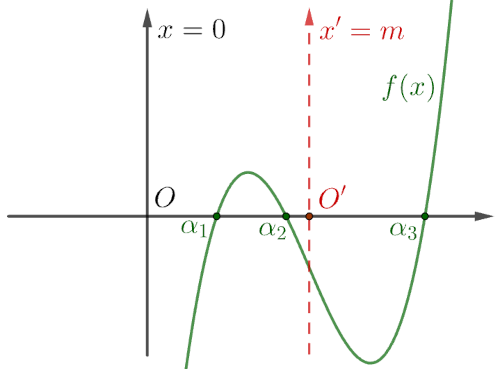
Answer: The aforementioned theo-rem of symmetric polynomials (Vi-eta) also applies to the cubic equa-tion:

$$ f(x) = ax^3 + bx^2 + cx + d = 0, $$

where we can write:

$$ f = a(x-\alpha_1)(x-\alpha_2)(x-\alpha_3), $$

when we know the solutions α₁, α₂ and α₃. These remain if we divide the equation by a ≠ 0, so we get a new function g(x) = f(x)/a and a cubic equ-ation with the new notation x³ + a'x² + b'x + c' = 0 with the same previous solutions. The figure on the left shows the graph f, if the coefficients are real numbers then all three solutions (as in the figure α₁, α₂ and α₃) are real num-bers, otherwise it is possible for one of them to be real (let it be α₁ ∈ ℝ) with the other two conjugated to complex numbers (α₃ = α₂^*). In any case, the mean value of the solution is m = (α₁ + α₂ + α₃)/3.

1. When we slide the origin along the abscissa, O → O' for the mean value m, when x' = x + m, or x = x' - m, we get:

f(x' - m) = a(x' - m)³ + b(x' - m)² + c(x' - m) + d =
= a(x'³ - 3x'²m + 3x'm² - m'³) + b(x'² - 2x'm + m²) + c(x' - m) + d
= ax'³ + (-3am + b)x'² + (3am² - 2bm + c)x' - am³ + bm² - cm + d
= a[x'³ + (-3m + a')x'² + (3m² - 2a'm + b')x' + (-m³ + a'm² - b'm + c')],

x'³ + (-3m + a')x'² + (3m² - 2a'm + b')x' + (-m³ + a'm² - b'm + c') = 0,

where a' = b/a, b' = c/a and c' = d/a, where a ≠ 0 because the equation is cu-bic. However, 3m = α₁ + α₂ + α₃ = a', because the solutions for f and g are the same, so the term along x'² of this equation vanishes. Hence the given cubic equation becomes:

x'³ + px' + q = 0,

with coefficients p = 3m² - 2a'm + b' and q = -m³ + a'm² - b'm + c'. Its soluti-ons are some numbers β₁ = α₁ - m, β₂ = α₂ - m and β₃ = α₃ - m, which we use to define its Vieta coefficients:

s₁ = -β₁ - β₂ - β₃ = 0,
s₂ = β₁β₂ + β₁β₃ + β₂β₃ = p,
s₃ = -β₁β₂β₃ = q.

Let us show that these solutions (betas) can be expressed in terms of ss, that is, that they are symmetric, which is in accordance with the symmetric polyn-omial theorem.

2. Let's put x' = u + v, so we have:

(u + v)³ = u³ + 3u²v + 3uv² + v³ = (u³ + v³) + 3uv(u + v),
(u + v)³ - 3uv(u + v) - (u³ + v³) = 0,
p = - 3uv,     q = - (u³ + v³),
x'³ + px' + q = 0.

Hence it is:

$$ u^3 + v^3 = -q, \quad u^3v^3 = -\frac{p^3}{27}, $$

which are the Viete coefficients of the quadratic equation whose solutions are:

$$ u^3, v^3 = -\frac{q}{2} \pm \sqrt{\frac{q^2}{4} + \frac{p^3}{27}}. $$

But there are also solutions x'_1,2,3 = u + v to our cubic equation:

$$ \beta_{1,2,3} = \sqrt[3]{-\frac{q}{2} + \sqrt{\frac{q^2}{4} + \frac{p^3}{27}}} + \sqrt[3]{-\frac{q}{2} - \sqrt{\frac{q^2}{4} + \frac{p^3}{27}}}. $$

Since p and q are the Vieta coefficients of the cubic equation, and the solutions are expressed using them, the result is consistent with the symmetric polyno-mial theorem: solutions of the cubic equation can be expressed (by quadratur-es) with elementary symmetric (Vieta) polynomials.

3. For example, given a quadratic function:

f(x) = x³ - 7x² + 14x - 8.

Leading coefficient a = 1 so g(x) = f(x). We know m = (α₁ + α₂ + α₃)/3 = -7/3, the mean, sum value of the roots α₁, α₂ and α₃ which we are looking for indivi-dually. With (1) shifting x = x' + 7/3, we find:

f(x' + 7/3) = (x' + 7/3)³ - 7(x' + 7/3)² + 14(x' + 7/4) - 8 =
= x'³ + [-3(-7/3) + (-7/3)]x'² + [3(-7/3)² - 2(-7)(-7/3) + 14]x' +
+ [-(-7/3)³ + (-7)(-7/3)² - 14(-7/3) -8].

After a little calculation we find the cubic equation:

$$ x'^3 - \frac73x' - \frac{20}{27} = 0, $$

with coefficients:

$$ p = -\frac73, \quad q = -\frac{20}{27}. $$

which we include in (2) the solutions:

$$ x'_1 = \sqrt[3]{\frac{10}{27} + \sqrt{\frac{100}{27^2} - \frac{7^3}{27^2}}} + \sqrt[3]{\frac{10}{27} - \sqrt{\frac{100}{27^2} - \frac{7^3}{27^2}}} = $$ $$ = \sqrt[3]{\frac{10}{27} + \frac{\sqrt{3}}{3}i} + \sqrt[3]{\frac{10}{27} - \frac{\sqrt{3}}{3}i} $$ $$ = \frac13(\sqrt[3]{10 + 9\sqrt{3}i} + \sqrt[3]{10-9\sqrt{3}i}) = \frac53. $$

We have the factor ($x' - \frac53$) of the cubic function ($x'^3 - \frac73x' - \frac{20}{27} = 0$) and by dividing the polynomials we find the quadratic equation:

$$ (x'^3 - \frac73x' - \frac{20}{27}) : (x' - \frac53) \to x'^2 + \frac53x' + \frac49 = 0, $$

with the following two solutions:

$$ x'_{2,3} = \frac12(-\frac53 \pm \sqrt{\frac{25}{9} - \frac{16}{9}}) = -\frac13, \ -\frac43. $$

All three solutions of this cubic equation are the real numbers 5/3, -1/3 and -4/3. From x = x' + 7/3 it follows that the solutions x_1,2,3 = 4, 2 and 1 are the solutions of the given cubic equation (3). And its function is shown by the graph above, where α₁ = 1, α₂ = 2 and α₃ = 4.

4. Recall that the complex number z = x + iy, where x, y ∈ ℝ and i² = -1, and that its complex conjugate is z^* = x - iy. The conjugate sum is equal to the sum of the conjugates, (z₁ + z₂)^* = z₁* + z₂*, the conjugate product of numbers is equal to the product of the conjugates, (z₁ ⋅ z₂)^* = z₁* ⋅ z₂*, and the conjugate real number does not change. Hence, (z³ + pz + q)^* = z^*³ + p^* z^* + q^*, so if p, q ∈ ℝ, then z^* will be a solution of the cubic equation whenever z is a solution and its inverse, so one of the three solutions must be a real number.

The intensity, or modulus ∥z∥ = √(x² + y²) of a complex number z = x + iy, where x and y are real numbers and the imaginary unit is i² = -1, is its distance from the origin in the complex plane. Like vectors, they are subject to the tria-ngle inequality, each side of a triangle is no greater than the sum of the other two, and hence no less than their difference:

|∥z₁∥ - ∥z₁∥| ≤ ∥z₁ + z₂∥ ≤ ∥z₁∥ + ∥z₁∥.

We further see that for small moduli, ∥z∥ → 0, the polynomial tends to its free term, so the cubic function z³ + pz + q → q, and for large moduli the polyno-mial overshoots it. Somewhere between these two extremes, for some z₀, the equality will hold, for example z₀³ - (7/3)z₀ = 20/27. In short, this is also an explanation of the fundamental theorem of algebra (Vieta, 2), that every pol-ynomial has at least one solution.

Tours » srb

Question: How do you know that by increasing the modulus z the polynomial will reach its free term?

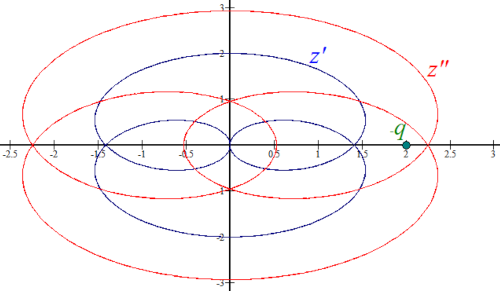
Answer: I suppose that the positivi-ty of the intensity ∥z∥ ≥ 0, from zero to over ∥q∥ is disturbing, say becau-se q can be a negative number, or inaccessible to modules. In the fig-ure on the right, the ℂ plane, we see the visits of the cubic complex expr-ession z³ - z, where z = re^iθ. In this case, r = 1 in the case of z' and r = 1.2 in the case of z'', and in both ca-ses the angles θ pass through all possible values. Here p = -1 and q = -2 cubic equation z³ + pz + q = 0, and we see that the blue rounds (z') do not add up to two (-q), but the red ones (z'') do. Somewhere in between is such a radius, 1 < r₀ < 1.2, of the complex number z₀ = r₀e^iθ (then the angle θ = 0) that exactly z₀³ - z₀ = 2. Notice that these angles describe the center three times to return z to the origin, because the cubic eq-uation has three solutions.

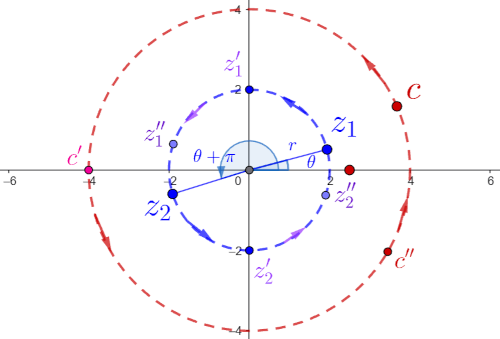
1. The figure on the left gives a sim-pler example of the approximation of the variable ∥z∥ = 2 and the con-stant ∥c∥ = 4, both in complex num-bers, and when z² = c. Both are co-mplex numbers z = 2e^iθ, c = 4e^iφ, where the angle φ = 4θ is the "co-nstant" c ∈ ℂ (it does not change the modulus, only the angle), so it circles twice as fast as the solutions of that quadratic equation (z₁, z₂) → (z'₁, z'₂) → (z''₁, z''₂). Here we notice that after going around, a full circle θ = 2π, the constant comes to the initial position (c'' → 4), but the solutions have switched places (z₁ ⇄ z₂).

This inconsistency in the order of the two solutions of the quadratic equation (Vieta, 3) is the cause of the appearance of roots in its solutions:

$$ z_{1,2} = \frac12(-a \pm \sqrt{a^2 - 4b}), $$

from z² + az + b = 0. Namely, while the expression under the root (a² - 4b) in the complex plane (ℂ) goes a full circle around the origin, the solutions change places; they need another circle of the variable to get to where they were. It is not possible to consistently insist on the order of solutions of a quadratic equ-ation.

2. We have seen (Cardano) how the general cubic equation reduces to the two-parameter form z³ + pz + q = 0. However, it always has three solutions (z₁, z₂ and z₃) which may be different. Then from (z - z₁)(z - z₂)(z - z₃) = 0, due to several arbitrary constants, the solutions z₁, z₂, z₁ ∈ ℂ, from the number of parameters, p and q, we see that a bijection between the solution and the parameters is not possible. A coincidence of this kind is resolved in a cubic equation by the dependence of the solution, say z₁ = a ∈ ℝ and z₃ = z₂^* ∈ ℂ, when:

(z - a)(z² + az + b) = 0,
z³ + (b - a²)z - ab = 0,
z³ + pz + q =0,

so p = b - a² and q = -ab. Hence it has the possibility of being solved by quad-ratures, which polynomial equations of the fifth degree and higher do not ha-ve.

3. Quartic equation (quartic):

f:     az⁴ + bz³ + cz² + dz + e = 0.

we assume rational coefficients (a, ..., e ∈ ℚ). It is solved similarly to the cubic but much more complicated. Its four solutions are either four real numbers, e.g. (z - 1)(z - 2)(z - 3)(z - 4) = 0, or conjugate complex numbers, or mixtures of both. With rational coefficients, the quartic equation will have pairs of con-jugate complex solutions; there is no single complex with three reals, nor th-ree complex with one real solution. They are with $\binom{4}{2} = 6$ symmetry, that is, three pairs of semi-symmetric products:

(α₁ + α₂)(α₃ + α₄) = β₁,
(α₁ + α₃)(α₂ + α₄) = β₂,
(α₁ + α₄)(α₂ + α₃) = β₁.

Let's form a cubic equation with solutions to these beta functions:

g:     (z - β₁)(z - β₂)(z - β₃) = 0,

it is completely symmetric. Its solutions can be obtained by quadrature, which means that they can be expressed in terms of Vieta coefficients. Introducing the shift z' = z - b/4a in f, it becomes:

f ':     z⁴ + pz² + qz + r = 0

with the first Vieta coefficient zero, α'₁ + α'₂ + α'₃ + α'₄ = 0. Then we have:

β'₁ = (α'₁ + α'₂)(α'₃ + α'₄) = (α'₁ + α'₂)(-α'₁ - α'₂) = -(α'₁ + α'₂)²,
α'₁ + α'₂ = √(-β'₁),

and then, in any way, we can also find solutions (alpha) of the fourth degree equation expressed by radicals. In short, this would be the procedure of Lag-range (1770) in the time before group theory and Galois, by which he consi-dered why there is no general solution to quadratures of fifth degree equati-ons.

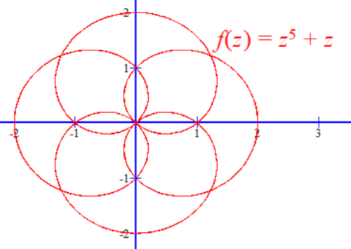
4. In the figure on the right are all positions of the complex function f(z) = z⁵ + z in the plane ℂ, variab-les z = e^iθ ∈ ℂ, angles θ ∈ [0, 5⋅2π]. If z = 1 is f(z) = 2. When z = e^iπ/6, then f(z) = i. If z = e^iπ/3 yet f(z) = 1, and so on. When z traverses one fu-ll circle, 2π, the function f(z) draws five of them, 5⋅2π. Four immediate ones and the fifth one they descri-be. Every point C ∈ ℂ of the trajec-tory f(e^iθ) of that complex plane solves some equation z⁵ + z = C, when |z| = 1, but note that the symmetry, or interchangeability of some of its solutions, holds.

For a fixed |C| ≤ 2, we have up to five possible ones, say C ∈ {-2, -1, 0, 1, 2} al-ong the abscissa, each of which has up to four more complex solutions, but we cannot put some in front of others. This lack of order of solutions is the point of the lack of general solutions in quadratures of equations of the fifth degree and higher. Finally, with the equation of the fourth degree, the possibilities of quadratures are exhausted.

5. Whenever we have some symmetries, we can also look for the correspondi-ng conservation laws, the mapping of something into the same. Considering the bijections of mathematics and the truths of physics (Intellect, 1), symme-tries tell us about reality, that is, about observable, permanent and true phe-nomena. Hence all this attention to groups, fields and Galois theory, because it is close to (my) information theory.

Automorphism » srb

Question: What should you know about automorphism in Galois theory?

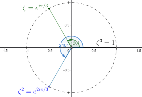
Answer: In short, a field is a group for both its operations, addition and multiplication (closed, associ-ative, commutative, with a neutral and an inverse element). Of interest to us are the field of rational numb-ers ℚ and its extensions ℚ(√2), ℚ(i), ℚ(√2, i) and the like. In the figure on the left is the field of ℝ(ζ), or the circle of the complex plane.

An automorphism of a field ℱ is a mapping ϕ : ℱ → ℱ that preserves additions and multiplications, if ϕ(a + b) = ϕ(a) + ϕ(b) and ϕ(a ⋅ b) = ϕ(a) ⋅ ϕ(b) holds for all a, b ∈ ℱ. In short, an automo-rphism ϕ of a field ℱ ⊇ ℚ is a mapping that preserves the structure and does not change the elements of ℚ, we say fixes them. The automorphisms ℱ ⊇ ℚ form a group called the Galois group of ℱ and denoted Gal(ℱ).

1. For example, the extension of the field of rational numbers ℚ is the field:

ℚ(√2) = {a + b√2 | a, b ∈ ℚ},

with only two automorphisms, the unitary mapping e(q) = q for all q in ℚ(√2) and ϕ(a + b√2) = a - b√2 for all a, b ∈ ℚ. The first is obvious, but the second easily follows from the definition of the automorphism field:

ϕ[(a₁ + b₁√2) + (a₂ + b₂√2)] = ... = (a₁ + a₂) - (b₁ + b₂)√2,

ϕ[(a₁ + b₁√2) ⋅ (a₂ + b₂√2)] = ... = (a₁a₂ + 2b₁b₂) - (a₁b₂ + a₂b₁)√2.

A field with two automorphisms has dimension two. The set of all automorp-hisms of the field ℱ forms a group under compositions. When ℱ is an exten-sion of ℚ, the group of automorphisms of ℱ is the Galoa group of label Gal(ℱ). In the case of ℚ(√2) this group is denoted C₂, since it has only two automorp-hisms, identical e and ϕ.

2. Let us assume an automorphism ϕ : ℱ → ℱ of the field ℱ which is some extension of ℚ, and prove that ϕ(x) = x for every x ∈ ℚ.

Proof: Suppose that ϕ(1) = x. It is clear that x ≠ 0, because:

ϕ(2) = ϕ(1 + 1) = ϕ(1) + ϕ(1) ≠ 0,

otherwise ϕ would map every number to zero, which is not an automorphism. Then:

x = ϕ(1) = ϕ(1⋅1) = ϕ(1)ϕ(1) = x²,
x = ϕ(1) = ϕ(1⋅1⋅) = ϕ(1)ϕ(1)ϕ(1) = x³,
...
x = xⁿ for all n > 1,

so since x ≠ 0, nor is it -1, it must be x = 1. Therefore, ϕ(1) = 1, and hence it easily follows from the definitions that ϕ(x) = x when x ∈ ℚ. ∎

3. Let us show that √2 ∉ ℚ in the extension of rational numbers ℚ(√2).

Proof: Suppose √2 ∈ ℚ. According to the previous (2) then ϕ(√2) = √2, and this contradicts this automorphism, ϕ(√2) = -√2. This means that the assu-mption is false and that √2 ∉ ℚ. ∎

4. An interesting extension of ℚ(√2) of ℚ is ℚ(√2)(i), where i² = -1, which we also denote by ℚ(√2, i). The element of that field is (a, b ∈ ℚ(√2)):

a + bi = (a' + b'√2) + (a'' + b''√2)i =
= (a' + a'') + b'√2 + a''i + b''√2i,

where a', a'', b', b'' ∈ ℚ. In addition to the identical automorphism ϕ₀ = e, there are three more:

ϕ₁(√2) = -√2,     ϕ₁(i) = i,
ϕ₂(√2) = √2,     ϕ₂(i) = -i,
ϕ₃(√2) = -√2,     ϕ₃(i) = -i.

Because of these four possibilities, such a group Gal(ℚ(√2, i)) is Klein V₄.

5. It is instructive to consider the field ℚ(∛2) = {a + b∛2 | a, b ∈ ℚ}, which has the base {1, ∛2, ∛4}, where the added, third term ∛4 = (∛2)² is also not a rati-onal number (nor ∛2), it cannot be obtained by adding the previous ones but only by squaring. As with the basis of vectors, linear independence is required to count the elements of the base, and the field ℚ(∛2) has three such elements. This means that the extension ℚ to the field of real numbers ℝ has an infinite base.

6. Finally, let us consider the smallest extension of the field ℱ over ℚ that con-tains all the roots of the polynomial f(z) = z³ - 2. Let us say that in the figure above there is a complex plane with only rational coordinates and cube roots of unity (ζ³ = 1):

$$ \zeta = e^{\frac{2\pi i}{3}}, \quad \zeta^2 = e^{\frac{4\pi i}{3}}, $$ $$ \zeta = \cos\frac{2\pi}{3} + i\sin\frac{2\pi}{3}, \quad \zeta^2 = \cos\frac{4\pi}{3} + i\sin\frac{4\pi}{3}, $$ $$ \zeta = -\frac12 + i\frac{\sqrt{3}}{2}, \quad \zeta^2 = -\frac12 - i\frac{\sqrt{3}}{2}. $$

They are the three roots of the polynomial g(z) = z³ - 1 = (z - 1)(z² + z + 1). Now we can write the roots of f as z1 = ∛2, z2 = ζ∛2 and z3 = ζ²∛2.

Note that z₂³ = (ζ∛2)³ = 2 and also z₃³ = (ζ²∛2)³ = ζ⁶∛8 = 2. Unlike 1, ζ and ζ² which are all three at a distance of 1 from the origin, the three points z₁, z₂ and z₃ are on their same lines but are ∛2 away from the origin. Therefore ℚ(z₁, z₂, z₃) is an extension of the field over ℚ, which contains all the roots of the poly-nomial f. However, ℱ = ℚ(i, ∛2) is the smallest extension of the field of ration-al numbers ℚ which contains the roots of the polynomial f(z) = z³ - 2. Namely, z₂ = ζz₁ and z₃ = ζz₂, but:

$$ -1 - \zeta = -1 - (-\frac12 + i\frac{\sqrt{3}}{2}) = -\frac12 - i\frac{\sqrt{3}}{2} = \zeta^2, $$

or 1 + ζ + ζ² = 0, i.e. there is a linear dependence of the vector, root 1, ζ and ζ², so we do not need ζ².

7. The broader physical and cosmic application of these abstract items lies in the "unreasonable effectiveness of mathematics" (Wigner, 1960). The first-degree equation ax + b with rational coefficients a, b ∈ ℚ has all solutions in the field of rational numbers. The second-degree equation ax² + bx + c = 0 already needs a slightly wider field ℚ(i, √q), with all q ∈ ℚ. The cubic also ne-eds third roots, and for the fifth degree no quadratures are sufficient. Here, where truths in general, including the known mathematical ones, are conside-red the foundation of reality, this concept is more than a metaphor. Truth is an infinite harmony, only fragments of which we can perceive with our limited perceptions, and unlike lies that conflict, each part of it is insufficient for us. Whatever door of its whole we open, we will find ourselves facing the next un-known exits, because the characteristic of reality is the connection of percepti-ons. This is just a harbinger of future complications.

Lattice » srb

Question: What is the fundamental theorem of Galois theory?

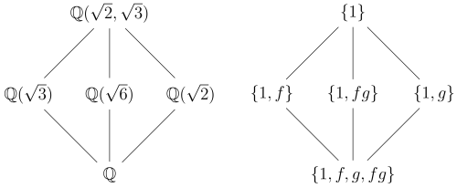
Answer: I will explain, but first let me quote it. Given a mapping s ∈ ℤ[x] and let F be a splitting field s, and G be a Galois group. Then the following holds:

1. The lattice subgroup G is identical to the lattice subgroup F, but inverted. Moreover, the subgroup H is normal to G, denoted by H ⊲ G, if the corresponding subfield is a normal extension of the field ℚ.
2. Given an intermediate field K, when ℚ ⊂ K ⊂ F, the corresponding subgroups H < G contain exactly those automorphisms that fix K.

Here ℤ[x] is the set of polynomials of the variable x and integer coefficients, ℤ = {..., -2, -1, 0, 1, 2, ...}, but for the basic field we take rational numbers from the set ℚ = {m/n | m, n ∈ ℤ, n ≠ 0}.

1. In the image above, on the right, on the left is a grid with extensions of the base field:

ℚ(r) = {a + b⋅r | a, b ∈ ℚ, r = √2, √3, √6},
ℚ(√2, √3) = {a + b√2 + c√3 | a, b, c ∈ ℚ}.

On the right is the lattice of the Galo group G, with automorphisms of those extensions:

e:   x ∈ ℚ(r) → x ∈ ℚ(r), or 1, identical mapping,
f:   x ∈ ℚ(√3) → x ∈ ℚ(-√3), conjugation √2 → -√2,
g:   x ∈ ℚ(√3) → x ∈ ℚ(-√3), conjugation √3 → -√3,
fg:   x ∈ ℚ(√2, √3) → x ∈ ℚ(-√2, -√3), conjugation of both.

Galois's theorem first says that these two lattices are equivalent when placed upside down, like in that picture.

2. An example of the field F = ℚ(√2, √3) is the polynomial x⁴ - 5x² + 6, or as (x² - 2)(x² - 3) which is further factored (x - √2)(x + √2)(x - √3)(x + √3) = 0, into a fourth degree equation with solutions ±√2 and ±√3. It is an extension of ℚ and has four automorphisms: the identical mapping (in the image labeled 1), then the two mentioned f and g, and their composition fg. There are no more of them.

From this preservation of the field structure we find ϕ(√2)⋅ϕ(√2) = ϕ(√2⋅√2) = ϕ(2) = 2. In the previous answer it was proved ϕ(q) = q, for all q ∈ ℚ. However, if it were ϕ(√2) = √3, it would be ϕ(√2)⋅ϕ(√2) = √3⋅√3 = 3, i.e. a contradiction 2 = 3.

3. The previous article also states that the extension F of the field ℚ is and thus the Galois group of automorphisms of that F is Gal(F). The field of automorp-hisms (such as 1, f, g and fg of F) forms a group that is central to Galois theo-ry. The normal subgroup H of a Galois group G is one that is invariant under conjugation to all elements of the group, which means gHg⁻¹ = H for all g ∈ G. We write H ⊲ G. An extension into the field E of the field F is called “normal” if it is a splitting of the field of some polynomial. And the “divisible” field of the polynomial φ ∈ ℤ[x], with integer coefficients (ℤ is not a field) and with roots r₁, r₂, ..., r_n, is the field ℚ(r₁, r₂, ..., r_n).

The splitting field F of the polynomial φ(x) is the smallest field that has all the listed roots. It is also the smallest field in which φ(x) is divided into factors as (x - r₁)(x - r₂)...(x - r_n) ∈ F[x]. As a reminder, the Galois group of the extension F ⊇ G is the group of automorphisms of F, which we denote by G(F).

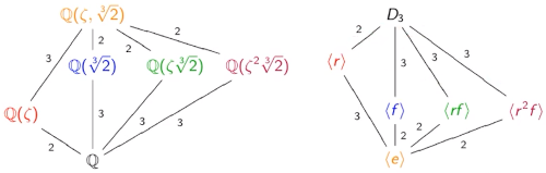
4. The video attachment of the ima-ge on the left will be a little clearer to you than the Wikipedia image above. On the left is the lattice of the subfield ℚ(ζ, ∛3), and on the right is the lattice of the subgroup Gal(ℚ(ζ, ∛3)). We are talking about the solutions of the polynomial x³ - 2 = (x - ∛2)(x² + x∛2 + ∛4), i.e. irrational ∛2, ∛4, complex ζ = exp(2i\pi/3), ζ² = exp(4i\pi/3) and the integer 1, which form a base of 2⋅3 = 6 elements.

For example, the number on the connector ℚ—2—ℚ(ζ) speaks of two linearly independent numbers, vectors 1 and ζ = -1/2 + i√3/2. Note that ζ² = -1 - ζ and such linearly depends on them. The number on the connector ℚ(ζ)—3—ℚ(ζ, ∛2) also speaks of the basis vectors of that extension: 1, ∛2 and ∛4. These th-ree are linearly independent, there is no a, b, c ∈ ℚ which are not zero, such that a⋅1 + b⋅∛2 + c⋅∛4 = 0. On the right side in the same figure are the corre-sponding automorphisms connected from top to bottom. The normal extensi-ons of the field ℚ are ℚ, ℚ(ζ) and ℚ(ζ, ∛2). On the right are the normal subgro-ups of D₃ such as: D₃, ⟨r⟩ and ⟨e⟩.

5. All this is important because of the following. The group G is “solvable” if there exists a chain of subgroups {e} = N₀ ⊲ N₁ ⊲ ... ⊲ N_n-1 ⊲ N_n = G such that each of the extensions N_k/N_k-1 is an abelian, commutative group. It is conven-ient to represent Galois groups by permutations and thus make them easier to check. But this is a separate topic whose "solvability" includes, for example, the proof that polynomials of the fifth degree and higher are not in general so-lvable by radicals, or that using only a ruler and compasses it is not possible to derive the geometric construction of the trisection of an angle. Here are also the answers to some difficult coding questions, but (we will see later) also the impossibility of communication of some subjects.

Extensions » srb

Question: What are "normal" extensions?

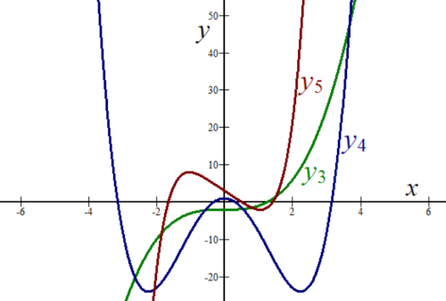
Answer: The image on the right sh-ows the graphs of three polynomia-ls in coordinate system Oxy:

y₃(x) = x³ - 2,
y₄(x) = x⁴ - 10x² + 1,
y₅(x) = x⁵ - 6x + 3.

The first (green) equation y₃ = 0 has three solutions ∛2, ∛2ζ and ∛2ζ² with the first real irrational, and the second and third are -1/2 ± i√3/2, which are conjugate complex num-bers. The second (blue) y₄ = 0 has all four solutions ±(√3 ± √2) irrational, and the third (red) of the fifth degree, y₅ = 0, is with two conjugate complex solu-tions and three real ones, without a general quadrature notation. The extensi-on ℚ → ℚ(∛2) contains one solution of the cubic (y₃) but not all, while the ex-tension ℚ → ℚ(√2, √3) includes all solutions (y₄), a fourth-degree polynomial, and is therefore called its normal extension.

1. Let F ⊂ E be the extension of the field and p ∈ E[t] be a monic polynomial, meaning one variable t and coefficients from E, of the nth degree:

p(t) = a_ntⁿ + a_n-1t^n-1 + ... + a₁t + a₀ = 0,     a_n, ..., a₀ ∈ E.

We say that p splits over E if there exist elements β₁, β₂, ..., β_n ∈ E, which are all roots of the polynomial p, such that p(t) = a_n(t - β₁)(t - β₂)...(t - β_n). It is the splitting over E of all n roots p belonging to E. Usually we take polynomials with integer coefficients ℤ[x] of a variable that is from the smallest field, x ∈ ℚ, so in case the polynomial has roots outside that field we expand ℚ to their values, so if the wider field contains all the roots of the given polynomial, we call that field its normal.

2. In the examples in the picture, y_3,4,5 ∈ ℤ[x], but the integers ℤ ⊂ ℚ are not field, but the smallest field E of the set of rational numbers ℚ is. In the case of a cubic (y₃) function, the first extension is, say, ℚ(∛2) = {a + b∛2 | a, b ∈ ℚ} is also a field, but it is not normal, because it does not contain all the roots of its polynomial. According to the Eisenstein's criterion of irreducibility, the given polynomial has only two factors in the field ℚ(∛2) and the equation x³ - 2 = (x - ∛2)(x² + x∛ + ∛4) = 0. The first factor has the solution β₁ = ∛2 ∈ ℝ, and the second factor adds two more that we find by solving it as a quadratic equation (Vieta, 3):

$$ ax^2 + bx + c = 0, \quad a = 1, \; b = \sqrt[3]{2}, \; c = \sqrt[3]{4}, $$ $$ x_{1,2} = \frac{-b \pm \sqrt{b^2 - 4ac}}{2a} = \frac{-\sqrt[3]{2} \pm \sqrt{\sqrt[3]{4} - 4\sqrt[3]{4}}}{2}, $$ $$ x_{1,2} = (-\frac12 \pm i\frac{\sqrt{3}}{2})\sqrt[3]{2} = \sqrt[3]{2}e^{\pm 2\pi i/3}, $$

e.g.

$$ \beta_{3,4} = \sqrt[3]{2}e^{\pm 2\pi i/3} \in \mathbb{C}, $$

namely:

$$ \beta_1 = \sqrt[3]{2}, \; \beta_2 = \sqrt[3]{2}\zeta, \; \beta_3 = \sqrt[3]{2}\zeta^2, \quad \zeta = e^{2\pi i/3}. $$

Only with all three solutions would the extension of that polynomial be "normal". This would be an extension of the extension ℚ(∛2)(ζ) = ℚ(∛2, ζ) which would have, say, the following basis {1, ∛2, ∛4, ζ, ζ∛2, ζ∛4}. The el-ement ζ² = -1 - ζ, linearly dependent on the previous ones, is not a basis. Note that the same field ℚ(∛2, ζ) is also spaned by the basis {1, ∛2, ∛4, i, i∛2, i∛4}, where i² = -1.

3. We have obtained the normal extension of the given cubic equation, ℚ(∛2, ζ), which has four automorphisms: the identical e = σ₀ and three more:

σ₁(√2) = -√2,     σ₁(i) = i,
σ₂(√2) = √2,     σ₂(i) = -i,
σ₃(√2) = -√2,     σ₃(i) = -i.

An arbitrary element of that field represented by its base is:

$$ x = a + b\sqrt[3]{2} + c\sqrt[3]{4} + di + e\sqrt[3]{2}i + f\sqrt[3]{4}i, $$

so let's see what we get with consecutive automorphisms:

○	σ0	σ1	σ2	σ3
σ0	σ0	σ1	σ2	σ3
σ1	σ1	σ0	σ3	σ2
σ2	σ2	σ3	σ0	σ1
σ3	σ3	σ2	σ1	σ0

For example, σ₂ ○ σ₃(x) =

$$ \sigma_3\circ \sigma_2(a + b\sqrt[3]{2} + c\sqrt[3]{4} + di + e\sqrt[3]{2}i + f\sqrt[3]{4}i) = $$ $$ = \sigma_3(a + b\sqrt[3]{2} + c\sqrt[3]{4} + di + e\sqrt[3]{2}i - f\sqrt[3]{4}i) $$ $$ = a + b\sqrt[3]{2} + c\sqrt[3]{4} + di - e\sqrt[3]{2}i + f\sqrt[3]{4}i = \sigma_1, $$ $$ \sigma_3\circ \sigma_2 = \sigma_1 $$

and similarly we find the other elements of the table. These automorphisms form an Abelian, commutative group called the Galois group of the given poly-nomial. It is closed to the composition of automorphisms which is associative, has a neutral element σ₀ and each is its own inverse (σ_k ○ σ_k = σ₀), and it is al-so Abelian, i.e. commutative. Since this is a polynomial of degree three, appli-cation of Galois theorems says that it can be represented by quadratures, wh-ich we have already done in the general case (Cardano).

4. A similar table is given by the automorphisms of a fourth-degree polynomi-al (y₄) whose normal extension is the field ℚ(√2)(√3) =

ℚ(√2, √3) = {A + B√3 | A, B ∈ ℚ(√2)} =
= {(a₁ + a₂√2) + (b₁ + b₂√2)√3} | a₁, a₂, b₁, b₂ ∈ ℚ}
= {a + b√2 + c√3 + d√6 | a, b, c, d ∈ ℚ}.

There are four automorphisms of this field, four conjugations ±√2 ± √3, and their Galois group has a composition table like the previous one and is also commutative. This possibility of solving by radicals is a common property of quadratic, cubic (degree 3) and quaternary (degree 4) equations, with the sa-me proof based on the commutativity of their Galois groups. In general, all polynomials, of any degree, when they have integer, rational, or real coeffici-ents, if they have a complex number z as a root also have a conjugate complex number z^* as a root. Namely, if a_nzⁿ + ... + a₁z + a₀ = 0, then:

(a_nzⁿ + ... + a₁z + a₀)^* = 0^*,
a_n(z^*)ⁿ + ... + a₁(z^*) + a₀ = 0.

Such equations have pairs of conjugate complex solutions, or individual real roots, which means that a fourth-degree equation, in addition to the four real solutions mentioned, has a pair of conjugate complex and a pair of real, or two pairs of complex conjugate roots. It is easy to see that this leads to tables of commutative groups like the one above, with solutions in radicals. That is the problem with equations of the fifth degree and higher, which are left without a general solution in radicals. Their Galois groups are not commutative.

Cyclic Group » srb

Question: Why would an automorphism of a group be noncommutative?

Answer: For example, Aut(ℂ, +) and its two automorphisms, the first conjugation z → z^* and mult-iplication by imaginary i. Then (iz)^* = -iz^* ≠ iz for z ≠ 0. No commutati-vity.

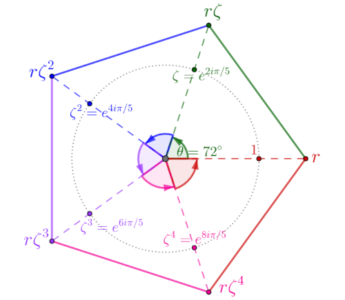
For another example, the image on the left is the cyclic group of order five (ℤ₅). This “fifth group” is the simple cyclic group ℤ₅ of integers modulo 5 under addition. The aut-omorphism is determined by map-ping the base 1. Since \(\mathbb{Z}_{5}\) is a prime number, each element of {1, 2, 3, 4, 5}, analogously to {1, ζ, ζ², ζ³, ζ⁴}, would be a generator.

There are five such possible mappings, automorphisms of the generator ζ and let σ(ζ) = ζ³. Then σ(ζ³) = σ(ζ)³ = (ζ³)³ = ζ⁹ = ζ⁴, then ζ⁴ → (ζ³)⁴ = ζ¹² = ζ², so ζ² → ζ^3⋅2 = ζ and the circle closes, the sequence of mappings repeats (Modu-lo). Otherwise, an Abelian group has a commutative automorphism group if and only if it is cyclic. However, if we extend ℤ₅ to a noncyclic group, its auto-morphism group immediately becomes noncommutative. For example, ℤ₂×ℤ₃, which we have in the case of the fifth degree polynomial y₅(x) = x⁵ - 6x + 3 and its Galois group, which had (Extensions) two conjugate complex and three real solutions. In the ℤ₂ frame the automorphism is the complex conjugation, and in ℤ₃ it would be a cyclic substitution.

We know that where there are conservation laws, there is some symmetry (Noether), but more than that, it makes sense to view other symmetries (be-yond classical physical analogies) as some conservations. For example, rotat-ional symmetry passes into a moment of inertia, once a wheel is set in motion it has a constant circular momentum until friction or some other force stops it. Translational motion (of light) is a series of ups and downs (electric and mag-netic) that, when separated, resemble reflections. Complex symmetries also have their analogies in some conservations, more abstractly speaking, but if they do not commute, they seem to us as if they were leaving the previous fra-mework, as if they were seeking a further extension of the field. An example is the noncommutativity of position and momentum (or energy and time), rela-tions of indeterminacy that speak of abandoning the consistency we know.

Commutativity corresponds to simultaneity, while non-commutativity dete-rmines time and gives it a pace. If the first describes processes in a "vicious circle", the second then speaks of a step out of them. In this wider, stepped process, one can again get stuck in a loop, that is, remain in a group (group-oidity, that the result of calculating any elements from a set is always in the same set), or within a vector space (spaned by a given basis). Let's say:

C = AB - BA,     C² = I,

$$ \begin{pmatrix} 0 & 1 \\ 1 & 0 \end{pmatrix} = \begin{pmatrix} 1 & 1 \\ -1 & \frac12 \end{pmatrix} \begin{pmatrix} \frac12 & 1 \\ -1 & 1 \end{pmatrix} - \begin{pmatrix} \frac12 & 1 \\ -1 & 1 \end{pmatrix} \begin{pmatrix} 1 & 1 \\ -1 & \frac12 \end{pmatrix}. $$

This is one way to simulate translational motion (of light) as alternating ups and downs (electric and magnetic) that, when separated, resemble reflections.

Thus, we arrive not only at the answer to the question “Why would an automo-rphism of a group be noncommutative?”, but also at why it has to be like this. It is the topic of my book “Multiplicity” (2018), and it also touches on Gödel's impossibility theorem (correctness is incomplete). Here's how. A field is clos-ed under addition and multiplication, and each of these two operations is co-mmutative for itself. Namely, a + b = b + a and b ⋅ c = c ⋅ b, for all elements a, b and c of that field, but their combinations will go outside that box like this, or similar a + b ⋅ c ≠ a ⋅ b + c. In the nature of these abstractions, there is alw-ays some open exit door, such as noncommutativity.

Euclid » srb

Question: Are geometric constructions a type of field?

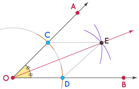
Answer: Geometric constructions with compass and straightedge wi-thout Euclid's division (Elements) are groups, but not fields, because operations with ruler and compass cannot be replaced, they are not commutative. The group is closed (to certain constructions), associa-tive, has a neutral and (each) inv-erse element, but in order to get to the bisector of the angle (figure on the right), if we have angle ∠AOB, we first open the compass OC and use a semicircle to transfer that length to OD ⊂ OB. Then, using the same compass, with centers at C and D, we draw circles that intersect at point E. The ray OE is the bisector of ∠AOB.

1. The ruler strokes connecting the given points were inspired by the stretchi-ng of a rope between two pegs by ancient Egyptian builders, while drawing a circle with a compass is equivalent to one of the workers walking around a st-ationary second while holding a taut rope. These analogies and the formalism of geometry were developed to incredible limits by the ancient Greeks from the following five postulates alone:

1. We can connect any two given points into a length.
2. A length (straight) extends indefinitely on both sides.
3. Given any point C and length r (radius, opening of the hexagon), a circle can be constructed around K(C, r).
4. All right angles (90°) are congruent.
5. If two lines intersect a third with interior angles less than right angles (α < 90° and β < 90°) they intersect on the sides of those angles.

We know the basic geometric constructions from high school, so I'll just list them here: the transfer of a line, the transfer of an angle, the construction of a line bisector, the construction of an angle bisector, the construction of a norm-al to a given line through a given point outside that line, the construction of a parallel to a given line through a given point outside that line. These are the seven basic constructions from which we derive all the others.

2. From the standpoint of Descartes's (1637) coordinate geometry, it is easier to see the limitations of Euclidean constructions. The equation of a straight line is of the first degree, y = kx + n, where k = tan(φ) is the slope of the line with respect to the abscissa for an angle φ, and n is the point where it interse-cts the ordinate. The crown K(C, r) is represented by the second degree equa-tion, (x - a)² + (y - b)² = r², with center C(a, b). By constructing a right angle, we define the abscissa (x-axis) and the ordinate (y-axis). By successively tran-sferring the initial length, which we declare to be the 1, and then by dividing these initial lengths (construction of the bisector of the line), we find 1/2, 1/2², ..., 1/2ⁿ, and build a coordinate system.

The coordinates we obtain in this way are an extension of the field of rational numbers ℚ, that is, the field ℚ(√q), where q ∈ ℚ. These are the solutions of the quadratic equations, ax² + bx + c = 0, with rational coefficients a, b, c ∈ ℚ:

$$ x = \frac{-b \pm \sqrt{b^2 - 4ac}}{2a}. $$

For example, there are no solutions to cubic and higher-degree equations, and no constructions that would reduce to such coordinates. Note that the moves that lead to these values, by construction using compasses and straightedge without division, are not commutative, but their results form a field. We can-not connect two points on a circle with a ruler if we have not first constructed the circle.

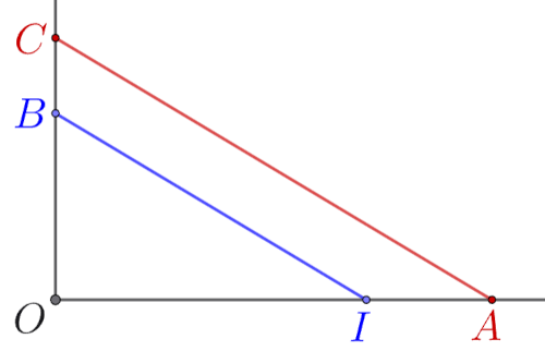
3. For example, we construct the product c = ab of the given lengths a = OA and b = OB by applying th-em to the arms of the right angle ∠AOB = 90° and the unit length 1 = OI ⊂ OA which can be shorter (as in the picture on the left) or longer than a. In any case, and we constr-uct the parallel AC ∥ IB, so from the similarity of the triangles we have:

OB : OI = OC : OA,

or b : 1 = c : a, i.e. c = ab. If we set the known OC = b and then the unknown OB = c, and keep OA = a, the same proportion gives c = b/a. Thus, with the given lengths a and b, we have constructed, first their product, then their quotient. We construct the rational numbers of the Cartesian plane.

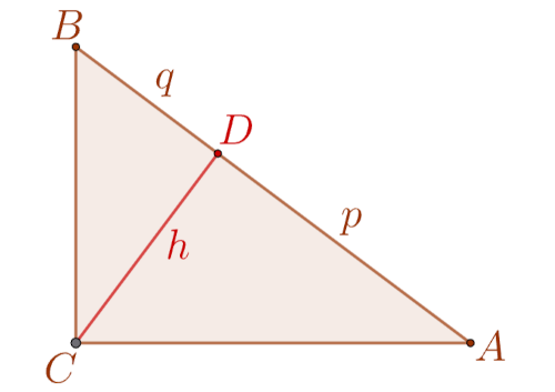
4. The figure on the right sketches the result of h = √p construction of the root of a given length p, when q = 1. The triangle ABC has a right angle ∠C = 90° and an altitude h = CD on the hypotenuse AB, which it divides into p = AD and q = DB.

The similarity of triangles CDA ∼ BDC gives h : p = q : h, and hence h² = pq, so if we choose q = 1 and p a given length, we get h = √p, the root of the given length. This shows that the roots of lengths p can also be constructed Euclideanally. According to the previous explanation, (h) are the roots of rational numbers (p).

We construct a unit length DB to the left of the origin and add to it the given length p = DA to the right of the origin of the abscissa. The midpoint of the sum of the lengths is the center S of the circle with radius r = (1 + p)/2 that intersects the ordinate at point C. This is a right angle of the triangle ABC, because the diameter is seen from the periphery of the circle at an angle of 90°.

5. For example, a regular heptagon cannot be constructed using only a comp-ass and a ruler without division, which automatically means that its central angle of 2π/7 = 360°/7 ≈ 51.43° cannot be constructed either. This impossibi-lity was mathematically proven in the 19th century thanks to the Gauss-Want-zel theorem on constructible polygons. From the above, we see that, for exam-ple, the cosine of that angle (the projection of the central distance) is not a so-lution to any quadratic equation with rational coefficients. One of the solutio-ns to the cubic equation 8x³ + 4x² - 4x - 1 = 0 is x = cos(2π/7).

Pentagon » srb

Question: Where are some basic geometric constructions with compasses and straightedge without division?

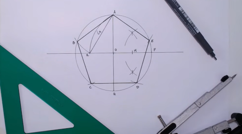
Answer: The picture on the left sh-ows a video of the construction of a pentagon, with some simpler ones in the appendix. Look at this your-self so we can find explanations. For example, it is puzzling why such a construction is possible at all, or why the center of the radius OM = OP/2 and MT₄ = MR give ℓ₅ = T₄R, i.e. the length of the side of the inscribed regular pentagon. And let's start from the golden ratio, which is φ = (1 + √5)/2 ≈ 1.618, in the next picture.

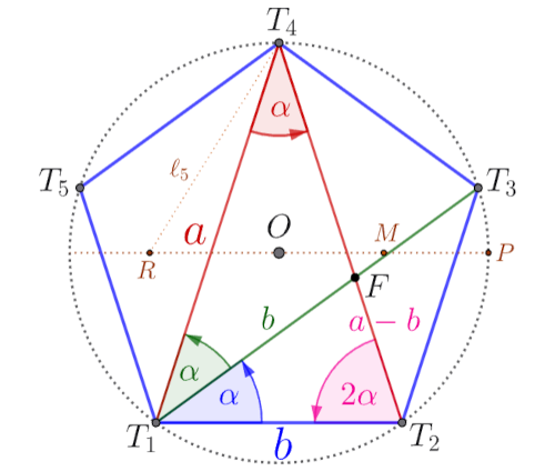
1. In the image on the right, all sides of the pentagon b = 1 with diagonals a that open equal angles α as peripheral angles that look into equal chords, so ∠(T₄T₂T₁) = 2α, then α = 180°/5 = 36°, because the sum of the angles of the triangle (T₁T₂T₄) is 180°. But T₁T₂ = T₁F = FT₄ = b, so the similarity of the tri-angles gives a : b = b : (a - b) and the square form a² - ab - b² = 0. From this follows the possibility of this construction (Euclid) and the value of the diagonal a = (1 + √5)/2 = φ, if b = 1, as a solution to that quadratic equation (Vieta).

2. Using the cosines theorem (b = 1, a = φ):

(T₁T₂)² = (T₁T₄)² + (T₄T₂)² - 2⋅(T₁T₄)⋅(T₄T₂)⋅cos(α),
1 = φ² + φ² - 2⋅φ⋅φ⋅cos(36°),
2⋅φ²⋅cos(36°) = 2⋅φ² - 1,

$$ \cos(36^\circ)= 1 - \frac12 \cdot \frac{1}{\varphi^2} = 1 - \frac12\left(\frac{2}{1 + \sqrt{5}}\right)^2 = $$ $$ = 1 - \frac{1}{3 + \sqrt{5}} = \frac{2 + \sqrt{5}}{3 + \sqrt{5}}\cdot\frac{3-\sqrt{5}}{3-\sqrt{5}} = \frac{1 + \sqrt{5}}{4}, $$

cos(36°) = φ/2,     sin(36°) = √[1 - (φ/2)²].

The cosine of an angle of 36° is equal to half the golden ratio, and the sine is given by the general formula cos²(α) + sin²(α) = 1.

3. When the radius of the circumcircle is one, OP = 1, also OT₄ = 1, and its half OM = 1/2. The Pythagorean theorem gives MT₄² = OT₄² + OM², i.e. MT₄² = 1² + (1/2)² = 5/4, and hence MT₄ = √5/2 = MR. Replacement, further, OR = MR - 1/2 = (√5 - 1)/2 = 1/φ. Namely, [(√5 + 1)/2]⋅[(√5 - 2)/2] = 1, or φ⋅(1/φ) = 1. The Pythagorean theorem again is ℓ₅² = (RT₄)² = (OR)² + (OT₄)², hence:

$$ \ell_5 = \sqrt{\frac{5 - \sqrt{5}}{2}} = 2\sin(36^\circ). $$

In the upper right image, let ON be ⊥ T₁T₂, so ONT₂ is a right triangle with side NT₂ = OT₂⋅sin(36°). When the circle of unit radius, OP = 1, then the side of the regular pentagon is b = 2⋅sin(35°) = ℓ₅. This proves the construction of the pentagon from the previous image (left) and a few more things along the way.

4. The intention of such a detailed explanation of the mathematics of the re-gular pentagon is not to just tell you high school topics, but to point out the (Hilbert space) arrangement of truths and lies that becomes familiar to us from machine learning models (LLM) when more frequent occurrences (to-kens) of phrases are metrically closer. For example, the word "cat" will be found closer to the word "dog" than to the word "tractor", because that is how it is in most common speech. This makes it easier to guess sentences because the more likely continuations are closer to the given space of those tokens. The abstract space of ways to construct a regular pentagon is similar to this. The above sequence of moves with a compass and a ruler without division is not the only possible one for constructing that pentagon, but even from such a small amount it is possible to recognize how easily it is possible to get lost and not complete the construction. What is outside the possible ways of solving the task, in this kind of information theory, I call the world of lies.

Quintic » srb

Question: Was Galois the first to prove that there is no general solution by ra-dicals for equations of the fifth degree?

Answer: No, before Galois (1830) it was proved by Abel (1824), and be-fore that by Cauchy (1813), who co-rrected or supplemented the proof of Rufi (1799). Even earlier, this pr-oblem was considered by Lagrange (1770) with symmetries, which I recently mentioned (Tours). I can explain that a little more.

Quadratic equations can have two solutions due to symmetry such that they are interchangeable. This follows from the description of the intensity ∥z(θ)∥ = 1, the simplest second-order equation z² = 1. We are talking about complex numbers, z = e^iθ, when the angle θ increases from 0 to 2π and beyond, but with an emphasis on the Lagrange method. While this complex number (vector) is circling the unit circle, its intensity does not change and, simply put, a single linear function (of the form ax + b) is not sufficient to describe its two solutions z_1,2 = ±1. The angle increases θ = 0, ±π, ±2π ..., and the solutions remain the same (i² = -1). This symmetry is reflected in the symmetry of the expressions s₁ = z₁ + z₂ and s₂ = z₁ ⋅ z₂ (Vieta), elementary symmetrical forms.

In the case of higher-order equations, say, with three solutions or in general three functions A, B, C, there are trinomials AAB + BBC + CCA and ABB + BCC + CAA with the property that no matter how we interchange the entries A, B and C, we will get the same functions we started with. You can invert them (as you would if you interchanged only A and B) or they can both stay in place (as you would when you rotated A to B and then to C), but in either case you get them back.

With four solutions, or four functions A, B, C and D, the analogy is made with the binomials AB + CD, AC + BD and AD + BC. No matter how you rearrange A, B, C and D, these three binomials remain the same collection. Galois would say that such permutations form a group, which is a more advanced version of Lagrange's reasoning. He noted that by putting AAB + BBC + CCA = p with ABB + BCC + CAA = q, we can have the general quadratic equation x² + px + q = 0 using the roots (A, B, C) of the cubic equation. In other words, the roots of the quadratic p and q are the bases of the roots of the cubic. Similarly, the roo-ts of the fourth degree equation (A, B, C,D) can be constructed using the roots of the third degree equation, with the symmetric forms AB + CD = p, AC + BD = q and AD + BC = r. In short, since a quadratic equation can be expressed in terms of radicals, it can also be expressed in terms of cubic (third degree) and then quartic (fourth degree) equations. However, there is no such analogy for the quintic (fifth degree).

Note that we are working with symmetries of Vieta forms. We can use them to represent the roots of the associated polynomial equations as well as symme-tric forms of that rank in general. This concerns the "fundamental theorem of symmetric polynomials". The simple reason why a fifth-degree equation is not solvable by quadrature in the general case is that there is no analogous set of four functions in A, B, C, D, and E that is preserved under permutations of those five letters.

Pover Sum » srb

Question: How do you know that Vieta coefficients can be used to define the roots of the associated polynomial equations and, in general, symmetric forms of that rank?

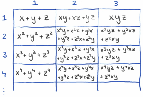
Answer: Of these questions, the first is trivial. For example, the equation:

x³ + e₁x² + e₂x + e₃ = 0

has Viete coefficients:

• e₁ = -(α₁ + α₂ + α₃)
• e₂ = α₁α₂ + α₁α₃ + α₂α₃
• e₃ = -α₁α₂α₃

where α₁, α₂ and α₃ are the solutions, the roots of the given cubic equation, such that:

(x - α₁)(x - α₂)(x - α₃) = 0.

So, these elementary symmetric functions e₁, e₂ and e₂ do indeed define the solutions of their cubic equation. It is understandable that the same obviou-sness applies to other polynomials.

1. The second question is explained by the attachment to the image on the rig-ht. The upper columns from left to right start with increasing factors of the in-dividual variables in the sums, and the margin rows from top to bottom have increasing exponents of the isolated sums of the variables. Let T[i, j] be the ith row and jth column of the table with index i, j ∈ ℕ, so the product of the ith element of the left margin and the jth title sum is:

T[i, 1] × T[1, j] = T[i+1, j] + T[i, j+1].

For example:

T[4, 1] × T[1, 2] = T[5, 2] + T[4, 3],

(x⁴ + y⁴ + z⁴)(xy + xz + yz) =
= x⁵y + x⁵z + x⁴yz + y⁵x + y⁴xz + y⁵z + z⁴xy + z⁵x + z⁵y,

with each sum of the sum degree i + j + 1. In that contribution, it is an intro-ductory explanation of Newton's theorem, that all polynomials obtained in this way are symmetric (do not change forms with the change of variables) and that they reduce to Vieta coefficients as to the sum of (the same) degrees of the given variables. Then one can see a sketch of the proof that the sums of the degrees of the variables themselves reduce to Vieta coefficients.

2. We don't have to go exactly in the direction of that video, but let's write:

α₁⁰ + α₂⁰ + α₃⁰ = s₀,
α₁¹ + α₂¹ + α₃¹ = s₁,
α₁² + α₂² + α₃² = s₂,
α₁³ + α₂³ + α₃³ = s₃,

where we easily recognize s₀ = 3 and s₁ = -e₁, and then we need to determine the sums of squares (s₂) and cubes (s₃) of the solutions (α₁, α₂ and α₃) of the given cubic equation. From (α₁ + α₂ + α₃)² = (α₁² + α₂² + α₃²) + 2(α₁α₂ + α₁α₃ + α₂α₃) is s₂ = e₁² - 2e₂ and then from:

α₁³ + e₁α₁² + e₂α₁ + e₃ = 0,
α₂³ + e₁α₂² + e₂α₂ + e₃ = 0,
α₃³ + e₁α₃² + e₂α₃ + e₃ = 0,

by adding we get s₃ + e₁s₂ + e₂ s₁ + e₃s₀ = 0, then:

s₃ = -e₁s₂ - e₂s₁ - e₃s₀ =
= -e₁(e₁² - 2e₂) + e₂⋅e₁ - e₃⋅3
= -e₁³ + 3e₁e₂ - 3e₃.

So:

s₀ = n = 3,     s₁ = e₁,     s₂ = e₁² - 2e₂,     s₃ = -e₁³ + 3e₁e₂ - 3e₃.

The sums of degrees 0, 1, 2, and 3 of the three roots of a given cubic equation are shown using only Vieta coefficients. These results apply to the quadratic equations, x² + e₁x + e₂ = 0, with appropriate coefficients and e₃ = 0.

3. The sums of higher powers of these roots will be found by recursion. We multiply the given cubic equation in turn by its roots and then add again to obtain s₄ + e₁s₃ + e₂s₂ + e₃s₁ = 0, where s₄ = α₁⁴ + α₂⁴ + α₃⁴, then:

s₄ = -e₁s₃ - e₂s₂ - e₃s₁ =
= -e₁(-e₁³ + 3e₁e₂ - 3e₃) - e₂(e₁² - 2e₂) + e₁e₃
= e₁⁴ - 4e₁²e₂ + 4e₁e₃ + 2e₂².

We also found the sum of the fourth powers. Again, multiplying the obtained forms of the cubic equation by its roots and adding all three, in the same way, we find s_k = α₁^k + α₂^k + α₃^k, for k ∈ ℕ, as a function of the Vieta values ​​e₁, e₂ and e₃, i.e. elementary symmetric polynomials.

4. These recursion steps are always preceded by finding the first sums by exponentiation. Let's look at this in the general example of a polynomial equation of degree n, for each n ∈ ℕ:

p_n(x) = xⁿ + e₁x^n-1 + ... + e_n-2x² + e_n-1x + e_n = 0,

where are now the Vieta coefficients:

• e₁ = -(α₁ + α₂ + ... + α_n)
• e₂ = α₁α₂ + α₁α₃ + ... + α_n-1α_n
• ...
• e₃ = (-1)ⁿα₁α₂...α_n

with α₁, α₂, ..., α_n solutions, i.e. roots of the polynomial p_n(x), for which the fundamental theorem of algebra also predicted the following form:

(x - α₁)(x - α₂)...(x - α_n) = 0.

This statement of the fundamental theorem of algebra (Vieta, 2) can also be found by looking at the changes in the intensity of the values ​​of ∥x∥, the mo-dulus of complex numbers up to the zeroing of the polynomial (Tours). We further use the notation:

s₀ = α₁⁰ + α₂⁰ + ... + α_n⁰,
s₁ = α₁¹ + α₂¹ + ... + α_n¹,
s₂ = α₁² + α₂² + ... + α_n²,
...,
s_k = α₁^k + α₂^k + ... + α_n^k,
...,

where it is easy to recognize s₀ = n and s₁ = -e₁, then we can also find the sums of squares (s₂), cubes (s₃), higher (s_k) solutions (α₁, α₂, ..., α_n) of the equation p_n(x) = 0. From:

(α₁ + α₂ + ... + α_n)² = (α₁² + α₂² + ... + α_n²) + 2(α₁α₂ + α₁α₃ + ... + α_n-1α_n)

we find s₂ = e₁² - 2e₂, so from:

(α₁ + α₂ + ... + α_n)³ = (α₁³ + α₂³ + ... + α_n³) - 3e₁e₂ + 3e₃,

it turns out s₃ = -e₁³ + 3e₁e₂ - 3e₃ and so on. We get a series of sums of powers:

s₀ = n,     s₁ = -e₁,     s₂ = e₁² - 2e₂,     s₃ = -e₁³ + 3e₁e₂ - 3e₃, ...,

whose terms reduce to Vieta coefficients. Optionally, in some step, at least n, such powers can be replaced by recursions. However, these powers are sym-metric polynomials and can be expressed in terms of the corresponding Vieta coefficients.

5. Symmetries are significant equivalences to conservation laws (of energy, spin, charge, and other known and unknown things). They express duration, i.e. constancy, they are also accurate when they are computable, i.e. functions, or problems or numbers that can be solved or calculated step-by-step followi-ng a clearly defined algorithm in a finite time and number of steps, they beco-me equivalent to the concept of reality as I use it here. That is why I dwell on them so much.

Pover Sum II » srb

Question: Can you give us a little more detail on the expressions for the sum of the powers of roots using Vieta coefficients?

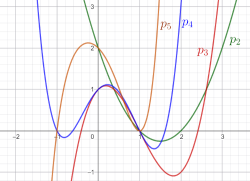
Answer: The image on the left has the graphs of four polynomials:

p₂(x) = x² - 3x + 2
p₃(x) = x³ - 3x² + x + 1
p₄(x) = x⁴ - x³ - 2x² + x + 1
p₅(x) = x⁵ - 2x² - x + 2

for testing results.

1. The Abel–Ruffini theorem states that general polynomials of degree five or higher cannot be solved by radicals, but the quintic equation of this form (p₅ = 0) is solvable. It factors into lower-degree polynomials:

x⁵ - x - 2x² + 2 = 0,
x(x⁴ - 1) - 2(x² - 1) = 0,
x(x² - 1)(x² + 1) - 2(x² - 1) = 0,
(x² - 1)[x(x² + 1) - 2] = 0,
(x - 1)(x + 1)(x³ + x - 2) = 0,
(x - 1)(x + 1)[(x³ - 1) + (x - 1)] = 0,
(x - 1)(x + 1)[(x - 1)(x² + x + 1) + (x - 1)] = 0,
(x - 1)²(x + 1)(x² + x + 2) = 0,
x₁ = x₂ = 1,     x₃ = -1,     x_4,5 = (-1 ±i√7)/2.

Since each root can be expressed using only integers with ordinary arithmetic operations and basic square roots, the equation p₅(x) = 0 is completely solvab-le by quadrature. I will also denote the roots of the equations by α_1..5 to avoid confusion.

2. We can solve the quartic equation (of the fourth degree) of the image like this:

x⁴ - x³ - 2x² + x + 1 = 0,
x⁴ - x² - x³ + x - x² + 1 = 0,
x²(x² - 1) - x(x² - 1) - (x² - 1) = 0,
(x² - 1)(x² - x - 1) = 0,
x₁ = 1,     x₂ = -1,     x_3,4 = (1 ±√5)/2.

The cubic, p₃(x) = 0, is even easier to factor:

x³ - 3x² + x + 1 = 0,
x³ - x² + x - x² + 1 - x² = 0,
x²(x - 1) - x(x - 1) - (x + 1)(x - 1) = 0,
(x - 1)(x² - 2x - 1) = 0,
x₁ = 1,     x_2,3 = 1 ± √2.

The quadratic equation, x² - 3x + 2 = 0, has solutions:

x₁ = 1,     x₂ = 2,

so let's start from it, in general such x² + e₁x + e₂ = 0, as the easiest. We know that e₁ = -α₁ - α₂ and e₂ = α₁ × α₂, because these are the Vieta coefficients giv-en to the roots of that equation, while we are looking for s_k = α₁^k + α₂^k respec-tively for k = 0, 1, 2, 3, ...

3. Since every polynomial equation can be uniquely assigned by Vieta coeffici-ents:

xⁿ + e₁x^n-1 + ... + e_n-1x + e_n = 0,
(x - α₁)(x - α₂)...(x - α_n) = 0,

this automatically means that its individual solutions can be defined by the same coefficients. Additionally, this means that the sums of the degrees of these solutions, s_k, are also (somehow) determined by the Vieta coefficients, and this means that it makes sense to look for such relations, expressions. With the equations p_n(x) = 0 we can start from the previous results (Pover Sum, 4):

s₀ = n,     s₁ = -e₁,     s₂ = e₁² - 2e₂,     s₃ = -e₁³ + 3e₁e₂ - 3e₃, ...,

$$ e_1 = -\sum_i \alpha_i, \quad e_2 = \sum_{i\lt j} \alpha_i\alpha_j, \quad e_3 = \sum_{i\lt j \lt k} \alpha_i\alpha_j\alpha_k, ... $$

setting α_k = 0 when k > n.

4. If we add both general quadratic equations (n = 2), each written with its solution, we get:

$$ \sum_{i=1}^2 (\alpha_i^2 + e_1\alpha_i + e_2) = 0, $$

s₂ + e₁s₁ + 2e₂ = 0,
s₂ - e₁² + 2e₂ = 0,
s₂ = e₁² - 2e₂,

which we already have for longer polynomials (n > 2), but now we establish that this is also true for quadratic ones. In the case of the quadratic equation in the figure, e₁ = -3 and e₂ = 2, with solutions α₁ = 1 and α₂ = 2, we get:

α₁² + α₂² = 1 + 4 = 5,     e₁² - 2e₂ = 9 - 4 = 5,

so that's also true, s₂ = 5.

5. When we multiply the previous quadratic equations by the solutions and add them together, we get:

$$ \sum_{i=1}^2 (\alpha_i^3 + e_1\alpha_i^2 + e_2\alpha_i) = 0, $$

s₃ + e₁s₂ + 2e₂s₁ = 0,
s₃ + e₁(e₁² - 2e₂) + e₂(-e₁) = 0,
s₃ = -e₁³ + 3e₁e₂,

which also fits the previous one, because e₃ = 0. That same quadratic (α₁ = 1 and α₂ = 2, with e₁ = -3 and e₂ = 2), gives:

α₁³ + α₂³ = 1 + 8 = 9,     -e₁³ + 3e₁e₂ = 27 - 18 = 9,

it is also true, s₃ = 9.

6. In the general case, k ∈ ℕ, since the Vieta coefficients (e₁ = -α₁ - α₂ and e₂ = α₁ ⋅ α₂) then the given quadratic equation (x² + e₁x + e₂ = 0) depend on the constant solutions (α₁ and α₂) will also be constants, so we use the well-known method of solving recursions:

s_k + e₁s_k-1 + e₂s_k-2 = 0,

r² + e₁r + e₂ = 0,

$$ r_{1,2} = \frac{-e_1 \pm \sqrt{e_1^2 - 4e_2}}{2}, $$

r₁ = α₁,     r₂ = α₂,

$$ \begin{cases} s_k = C_1\alpha_1^k + C_2\alpha_2^k, & \alpha_1 \ne \alpha_2 \\ s_k = (C_1 + C_2k)\alpha^k, & \alpha_1 = \alpha_2 \end{cases} $$

where the constants C₁ and C₂ determine the initial steps.

7. For example, in the first case (α₁ ≠ α₂):

s₁ = C₁α₁ + C₂α₂,     s₂ = C₁α₁² + C₂α₂²,
α₁ + α₂ = C₁α₁ + C₂α₂,     α₁² + α₂² = C₁α₁² + C₂α₂².

So, C₁ = C₂ = 1. Since α² + e₁α + e₂ = 0, these alphas are:

$$ \alpha_{1,2} = \frac{-e_1 \pm\sqrt{e_1^2 - 4e_2}}{2}, $$

so the general solution of the recursion, the sum of the kth powers of the root, is:

$$ s_k = \left(\frac{-e_1 + \sqrt{e_1^2 - 4e_2}}{2}\right)^k + \left(\frac{-e_1 - \sqrt{e_1^2 - 4e_2}}{2}\right)^k. $$

Simple, because s_k = α₁^k + α₂^k.

8. In the second case (α₁ = α₂ = α ≠ 0) is e₁ = -2α and e₂ = α², so we have:

s₁ = (C₁ + C₂)α,     s₂ = (C₁ + 2C₂)α²,
2α = (C₁ + C₂)α,     2α² = (C₁ + 2C₂)α²,
C₁ = 2,     C₂ = 0,
s_k = 2α^k = 2(-e₁/2)^k.

Note that the calculation of the recursion was trivial, redundant. Then apply it to other polynomials yourself, and if it doesn't work for you, I'll continue?

November 2026 (Original ≽)